
BFUT P19
Unification of Particle Physics: Deriving Fine Structure and Coupling Constants, W, Z, and Higgs Boson Masses, Redefining and Unifying Gravity and Time
Vijay Shankar Sharma
Independent Researcher, Gurugram, National Capital Region, India
vss@vijayshankarsharma.com
ORCID: 0009-0001-9622-6121
DOI: 10.5281/zenodo.20145567
The author declares no conflict of interest and no funding was received for this research.
License: CC BY-NC-ND 4.0
Abstract
The Big Flare-Up Theory (BFUT) treats the Spaticle field as the physical substrate from which particle and force sectors emerge. This paper develops the particle-sector consequences of the P16 condensation functional and the 3+e topology. It derives α_vss and αₛ_vss, the neutral core-stay resonance m_Z_vss = π⁴mₚ = 91.396 GeV/c², the charged n = 4 reconfiguration resonance m_W_vss = 256M = (256/3)mₚ = 80.066 GeV/c², and the resulting electroweak mixing quantity sin²θ_W_vss = 1 − (m_W_vss/m_Z_vss)² = 0.23257. The radial condensation mode is described by λ_H_vss = 2AR₀/π² and gives m_H_vss = 124.75 GeV/c². The W, Z, and H masses are therefore resonance outputs of the condensation architecture. The paper also develops time as substrate propagation, the DDR deformation-domain equation, and metric emergence from the carrier dynamics.
Paper 16 derives the adopted density through the particle-sector chain based on the proton charge radius and condensation geometry. The same value gives μₛ = 4.03358955 × 10⁻²⁷ m⁻¹, Lₛ = 2.47918135 × 10²⁶ m = 26.205 Gly, and aₛ = 1.20840317 × 10⁻¹⁰ m s⁻². Paper 18 [2] applies this aₛ without fitting it to 175 SPARC galaxies and KiDS-1000 lensing stacks. The SPARC results are 92.0 percent shape agreement, 98.8 percent flat classification, 14.3 percent non-flat classification, and a median outer relative residual of 0.096. The KiDS-1000 result is χ²/N = 9.78. These results connect the particle, galactic, and lensing sectors through one adopted substrate density.
Keywords: Standard Model; coupling constants; fine structure constant; strong coupling constant; electroweak mixing angle; W boson mass; Z boson mass; Higgs boson; substrate excitation resonances; deformation domain; gravitational carrier; time dilation; Spaticle field; cosmological constant; substrate density; ρₛ
1. Introduction
The Spaticle field condensation as the common substrate architecture from which forces, time, geometry, and particle resonances emerge.
This paper derives the fine-structure and strong-coupling relations from the P16 condensation geometry and develops the electroweak resonance chain from the same 3+e architecture. The Z and W masses are obtained independently; sin²θ_W_vss is then read from their squared mass ratio.
It also derives the quartic self-interaction coupling λₛ in its dimensionless form and λₛ in its SI form, the physical nature of time as substrate propagation, the full DDR deformation domain equation from the covariant carrier field equation F1-cov, the formal emergence of the metric tensor from substrate propagation structure, a unified propagation principle connecting gravity, inertia, time, and the speed of light, and a proof that the Spaticle substrate is Lorentz-compatible with no preferred drift frame.
Standard Model vs BFUT P19 framework: origin of coupling constants, number of free parameters, nature of time, and Higgs mass.
The standard model of particle physics is the most successful predictive framework in the history of science, calculating experimental outcomes to extraordinary precision [9]. But when one asks why the fine structure constant is 1/137 and not 1/140, or why the Z boson is heavier than the W boson, the standard model is silent. These quantities are experimentally measured and inserted into the equations by hand. They are brute facts, not derived quantities [9]. The standard model requires 19 to 26 such experimentally inserted free parameters with no derivation from a deeper physical substrate. The BFUT programme addresses this directly.
The BFUT framework does not replace the predictive machinery of quantum field theory. QFT remains an extraordinarily accurate description of how forces behave once they exist. BFUT proposes the underlying physical substrate that explains why the constants those forces depend on have the values they do. The distinction is between a calculating tool and a physical ontology: BFUT attempts to explain why the tool works, not to replace it [1][5].
Ontology Hierarchy in the BFUT Framework: the Spaticle field is the fundamental substrate. Its condensation topology produces organised particle and resonance modes; interactions arise as circulation asymmetries and deformation responses within the same substrate. Gravity, time, inertia, and causal limits are macroscopic manifestations of substrate propagation and relaxation. The metric tensor is the coarse-grained description of this propagation geometry. The electroweak H resonance is treated as a radial excitation of the condensation, not as a separate fundamental Higgs field.
Within BFUT, gravity, time dilation, inertia, and causal propagation are not independent postulates. They are four mechanical manifestations of one physical truth: that reality is entirely mediated through the finite propagation capacity of the Spaticle substrate. This is the unified propagation principle this paper formalises.
Standard General Relativity describes the source geometry and the curvature of spacetime with extraordinary precision, but it does not identify what physical entity is actually doing the curving. It is an extraordinarily accurate predictor of settled-domain geometry. BFUT P18 specifies the underlying local carrier: the Spaticle field substrate, whose mechanical deformation constitutes gravitation. This paper derives the coupling constants, the time-as-propagation account, and the metric-tensor emergence that complete the quantitative picture built on that carrier.
BFUT identifies a physical matter substrate that the author names the Spaticle field. Its adopted intrinsic equilibrium density is ρₛ = 7.3 × 10⁻²⁷ kg/m³ [3]. The field bends, compresses, waves, and becomes entrained by organised matter because it has a specific density. It is the physical substrate corresponding to what general relativity describes geometrically as spacetime.
The Spaticle field is not the luminiferous ether. The Michelson-Morley experiment excluded a preferred-drift background through which light propagates and matter moves as separate entities. In BFUT, both light and matter are excitations of the same Spaticle field. Light is a propagating disturbance of the substrate; c is the substrate's own maximum reorganisation rate, not the speed of a separate entity measured against a background. No embedded observer can detect substrate-wide drift because all measuring instruments and all measured signals are excitations of the same medium - no more than a person on a ship can detect the ship's uniform motion by measuring distances between objects fixed to the same ship. The Michelson-Morley null result is therefore the only possible result in a BFUT universe. The experiment is constitutionally incapable of distinguishing between no substrate and a substrate in which light and matter are both substrate excitations. The latter is the BFUT position. Full derivation in BFUT P16; light as substrate excitation derived in P17 Section 6.6 and P19 Section 13.
1.1 Symbols and Notation Used in This Paper
The following symbols are used throughout this paper. All values are from the BFUT Master Symbol Guide.
| Symbol | Definition | Value / Expression |
|---|---|---|
| Fundamental Spaticle Field Constants | ||
| ρₛ | Intrinsic equilibrium density of the Spaticle field | 7.3 × 10⁻²⁷ kg/m³ |
| Coupling Constants and Masses | ||
| α_vss | Fine structure constant | BFUT: 1/137.036655. Standard measured α = 1/137.035999. Difference: 0.00048% |
| αₛ_vss | Strong coupling constant | BFUT: 0.11785. Standard measured αₛ = 0.1179 at mZ. Difference: 0.043% |
| sin²θ_W_vss | Electroweak mixing angle | BFUT: 0.23257, obtained from 1 − (m_W_vss/m_Z_vss)². |
| m_W_vss, m_Z_vss | W and Z boson masses | m_W_vss = 256M = (256/3)mₚ = 80.066 GeV/c²; m_Z_vss = π⁴mₚ = 91.396 GeV/c². |
| m_H_vss | Higgs boson mass | λ_H_vss = 2AR₀/π² = 0.12903; v_vss = 245.565 GeV; m_H_vss = 124.75 GeV/c². |
| λₛ | Quartic Spaticle-field self-interaction coefficient | ρₛ/4 = 1.8257354 × 10⁻²⁷ kg/m³ |
| Shared Physical Constants | ||
| G | Gravitational constant | 6.674 × 10⁻¹¹ m³ kg⁻¹ s⁻² |
| c | Speed of light | 2.998 × 10⁸ m/s |
| ℏ | Reduced Planck constant | 1.055 × 10⁻³⁴ J·s |
| mₚ | Proton mass | 938.272 MeV/c² |
| rₚ | Proton charge radius | 0.8414 fm [CODATA 2018]. BFUT: R₀·ℓ_model = rₚ by construction. |
| ħ_vss | BFUT reduced Planck constant derived from P16 condensation geometry | mₚ·c·rₚ/(π·R₀) |
| R₀ | P16 free-energy minimum / dimensionless condensation radius | 1.27348 |
| ℓ_model | P16 physical condensation length scale | rₚ/R₀ |
| e | Elementary charge | 1.602176634 × 10⁻¹⁹ C |
| ε₀ | Vacuum permittivity | 8.8541878128 × 10⁻¹² F/m |
| m_e_vss | BFUT-derived electron mass | mₚ/(6π⁵) |
| m*_vss | BFUT particle-sector mass scale | m_e_vss/α_vss |
| rₑ_vss | BFUT electron length scale | α_vss ħ_vss/(m_e_vss c) |
| ug | Gravitational energy density at the particle scale | Gm_*²/(8πrₑ⁴) |
| uₛ | Spaticle field energy density | ρₛ c² |
| μₛ | BFUT equilibrium inverse length scale | 1/Lₛ |
| Lₛ | BFUT equilibrium screening scale | 1/μₛ = 26.205 Gly |
| λₛ | BFUT quartic Spaticle-field self-interaction coefficient | Dimensionless/SI forms used in P19 |
| J | P16 cooperation strength | 1.0 model units per co-rotating pair |
| Σ | P16 circulation imbalance measure | Σ(s) = Σᵢsᵢ |
| λcond | P16 imbalance penalty coefficient | 0.6 |
| αgeom | P16 geometric asymmetry coefficient | 0.5 |
| n | Number of condensation units | Integer unit count |
| k | Primary co-rotating group size | Integer group size |
| Dₛ | P16 circulation phase reward coefficient | 1.5 model units |
| φ | P16 circulation phase angle | 3+1: π/3; 4+0: 0 |
| sᵢ | Circulation sign of unit i | +1 or −1 |
| pairs(s) | Sum over products sᵢsⱼ for distinct pairs | Σ_{i<j}sᵢsⱼ |
| T₅ | Thermal disruption term | αT T|Ψ|² |
| αT | Thermal coupling coefficient | Defined in P19 thermal treatment |
| Ψ | Spaticle field amplitude/configuration | Field variable |
| Ψvac | Vacuum Spaticle-field amplitude | 2c |
| cs | Local effective substrate propagation speed | cs(x) |
| c₀ | Ambient vacuum propagation speed | c |
| η | Propagation efficiency | √(1−v²/c²) |
| γ | Lorentz factor reciprocal to η | 1/η |
| τc | Local constitutive response time | Defined by D-law |
| ξorg | Organisational coherence length | Effective domain-scale coherence length |
| Rd | Effective gravitational dominance radius | Structure-dependent |
| Meff | Effective gravitating mass | Derived within DDR extension |
| vrot | Rotational velocity | Structure-dependent |
| σₛ | Substrate surface/interface tension | Used in condensation energy terms |
| ωc | Condensation angular frequency | Used in rotational energy |
| Icond | Condensation moment of inertia | Used in rotational energy |
| m_eff | BFUT effective mode mass | Mode-dependent |
| c_s² | Local propagation-speed square | λₛ Φ²/ρₛ |
| aₛ | BFUT Spaticle acceleration scale | c√(Gρₛ/3) |
| T | Temperature | Thermal parameter |
| σ | Stefan-Boltzmann constant | Thermal radiation constant |
| u(T) | Thermal radiation energy density | 4σT⁴/c |
| E_unit | BFUT fundamental condensation energy unit | mₚc²/π |
| Vq | Core-unit volume | Three-sphere condensation volume |
| Vgap | Interstitial gap volume | Geometric gap volume |
| ρcond | Condensation-scale density | E_unit/(Vqc²) |
| E(n) | Total condensation energy for n units | −J·pairs(s)+λcond·Σ(s)²+(n−3)²+αgeom·(n−k)+Dₛ·cos(3φ) |
| E(μ) | Condensation energy with interstitial mass fraction | P16 functional evaluated at s=[+1,+1,+1,−μ] |
| μ | Interstitial mass fraction | 0.077 to 0.230 in the P19 physical range |
| a₀ | Bohr radius | ħ_vss/(m_e_vss c α_vss) |
| Kphys | Physical coefficient ℏc | 197.33 MeV·fm |
| L | Orbital angular momentum | n·ℏ |
| M | BFUT three-core mass scale | M = mₚ/3 = 312.757 MeV/c²; m_W_vss = 256M |
| λ_H_vss | BFUT electroweak radial coupling | 2AR₀/π² = 0.12903 |
| v_vss | BFUT electroweak radial scale | 6E_unit/α_vss = 245.565 GeV |
2. Adopted Substrate Density and Quartic Self-Interaction Coupling
Paper 16 derives the adopted substrate density through the following particle-sector chain [3]. The dimensionless free-energy functional uses A = 0.5, B = 0.56308, C = −1/3, and D = 1 and gives the stable minimum R₀ = 1.27348221.
Using the measured proton charge radius rₚ = 0.8414 × 10⁻¹⁵ m (CODATA 2018), the model length is ℓ_model = rₚ/R₀ = 6.607081 × 10⁻¹⁶ m.
The condensation geometry gives ħ_vss = mₚcℓ_model/π = 1.0545769 × 10⁻³⁴ J s, with mₚ = 1.6726219 × 10⁻²⁷ kg.
The electron mass follows as m_e_vss = mₚ/(6π⁵) = 9.1095552 × 10⁻³¹ kg.
The electromagnetic definition then gives α_vss = e²/(4πε₀ħ_vss c) = 0.007297318 = 1/137.036655.
The particle-sector mass scale is m*_vss = m_e_vss/α_vss = 1.2483430 × 10⁻²⁸ kg, and the electron length is rₑ_vss = α_vss ħ_vss/(m_e_vss c) = 2.8178873 × 10⁻¹⁵ m.
The gravitational energy density is ug = Gm*²/(8πrₑ⁴) = 6.5635567 × 10⁻¹⁰ J/m³. The factor 8πG is used because the Spaticle field is a matter substrate corresponding to what general relativity describes as spacetime. It bends, compresses, waves, and is entrained because it has density.
Mass-energy equivalence gives ρₛ = u_g/c² = 7.3 × 10⁻²⁷ kg/m³. This is the adopted value used throughout this paper.
A second route begins with the cosmological parameter Λ and uses ρ_Λ = Λc²/(8πG) = 3Ω_ΛH₀²/(8πG). This route is not adopted because it depends on H₀, which has multiple measured values and changes with cosmic epoch.
The adopted density fixes the quartic self-interaction coupling as λₛ = ρₛ/4 = 1.8257354 × 10⁻²⁷ kg/m³. It also fixes aₛ = c√(Gρₛ/3) = 1.20840317 × 10⁻¹⁰ m s⁻² for the DME equation of Paper 18 [2]. No fitted amplitude or exponent enters that equation.
Geometric derivation of the fine structure constant α and strong coupling constant αₛ from substrate condensation structure.
3. Strong Coupling Constant αₛ from Paper 16 Coefficients
The Paper 16 free-energy functional E(R) = A/R² + B·R² + C·R + D/R has four coefficients. A has a direct physical identification from the Schrödinger kinetic term: A = ħ_vss²/(2m_eff). As established in Paper 16 Section 5.4, Amodel = 1/2 exactly, independent of the numerical value of ħ_vss. B = 0.56308 (derived from void-filling geometry), C = −1/3 (derived, exact), D = 1 (derived, exact). All four coefficients are derived from first principles (P16 Appendix C). They confirm the stable interior minimum and the modular universality results of Paper 16 Section 21: The full binding-energy derivation and the robustness scans confirming this minimum across the parameter space are provided in Appendix A to this paper, kept as a separate file to preserve table formatting.
A = ħ_vss²/(2m_eff), B = ½ρₛ c_s² R₀², C = 4πR₀² σₛ, D = ω_c I_cond
where m_eff is the effective condensation mass, σₛ is the Spaticle field surface tension at the condensation boundary, ωc is the internal circulation frequency, and Icond = (2/5)m_eff R₀² is the rotational inertia of the three-core. The strong coupling constant at the condensation scale is the ratio of the inter-condensation binding energy to the substrate kinetic energy. After enforcing rotational invariance, substrate coherence, and dimensionless normalisation, the only surviving invariant combination of the condensation geometry is:
The structure A uniquely represents localisation energy, B uniquely represents substrate stiffness, and only this dimensionless ratio survives after normalisation. Using the derived values R₀ = 1.27348, B = 0.56308, A = 1/2:
The formula B × R₀⁴/A is the minimal surviving dimensionless invariant at the condensation scale. Dimensional closure requires dimensionless results; rotational invariance excludes non-scalar combinations; condensation topology requires expression in terms of stable-minimum parameters R₀ and the ratio B/A; and scale naturalness excludes combinations that diverge in the Newtonian limit. With derived values A = 1/2, B = 0.56308, R₀ = 1.27348, the dimensionless ratio is 2.962. The symmetry factor of the three-condensate geometry introduces an additional factor of 2 in the denominator, giving αₛ_vss = B·R₀⁴/(8π·A). Substituting A = 1/2, B = 0.56308, R₀ = 1.27348: αₛ_vss = 0.56308 × (1.27348)⁴/(8π × 0.5) = 0.11785. Measured at mZ: αₛ = 0.1179. Difference: 0.043%.
Asymptotic freedom emerges geometrically in this picture. As the probe scale shrinks, R₀ is compressed. The localisation cost A scales up rapidly while the bulk binding energy B × R₀⁴ decreases. The ratio αₛ_vss = B·R₀⁴/(8π·A) drops: asymptotic freedom is the geometric consequence of compressing the condensation vortex, not an algebraic sign convention. The stronger you squeeze the looser the internal grip. The full running derivation is given in the companion paper on particle physics coupling constants. [7][8]
The physical origin of the strong coupling follows from the interface energy. The binding energy density between two co-rotating condensations is ρₛ v²/2, where v = ω_c r_q. The free-condensation energy density is ρₛ c². Their ratio is ω_c²r_q²/(2c²), which is α_vss/2 at leading order. The numerical factor separating αₛ_vss from α_vss follows from three-sphere packing and the fraction of the condensation surface participating in binding. Decreasing the probe scale compresses the condensation and reduces the bulk binding-to-kinetic ratio, producing the weaker high-energy coupling.
The framework predicts different running behaviour for different interactions because distinct forces depend on different geometric properties of the condensation structure. Strong interactions depend sensitively on bulk condensation radius: compression shrinks R₀ and reduces the binding-to-kinetic ratio, weakening the coupling. Electromagnetic behaviour is tied primarily to internal rotational asymmetry, which is far less sensitive to overall volume under compression. This is why the strong coupling runs steeply with energy while the electromagnetic coupling barely changes: they respond to geometrically different properties of the same condensation structure under the same high-energy probe.
4. Fine Structure Constant α from Substrate Condensation Geometry
The fine structure constant is derived by substituting the BFUT expression for ħ into the standard electromagnetic definition. No additional step or new physical input is required beyond what is established in P16.
The standard definition is:
α = e² / (4πε₀ħc)
Substituting ħ_vss = mₚ·c·rₚ/(π·R₀) from P16 Section 5.2:
α_vss = e² / (4πε₀·[mₚ·c·rₚ/(π·R₀)]·c)
= e²·R₀ / (4ε₀·mₚ·c²·rₚ)
Substituting e = 1.602176634 × 10⁻¹⁹ C, ε₀ = 8.8542 × 10⁻¹² F/m, mₚ = 1.67262 × 10⁻²⁷ kg, c = 2.99792 × 10⁸ m/s, rₚ = 0.8414 × 10⁻¹⁵ m, R₀ = 1.27348:
α_vss = 1/137.036655
Measured: α = 1/137.035999 | Difference: 0.00048%
The inputs are e and c (exact), ε₀ and mₚ (measured), and rₚ = 0.8414 fm (CODATA 2018). Under the 2019 SI, ε₀ = e²/(2αhc), so this relation is the electromagnetic form of the condensation identity ħ = mₚcrₚ/(πR₀) of P16 Section 5.2: α_vss and ħ_vss reproduce α and ħ at the same 0.00048%.
The cross-check with R₀ confirms internal consistency. Solving the derived expression for R₀:
R₀ = 4ε₀·mₚ·c²·rₚ·α / e²
Substituting the measured value of α = 1/137.036 gives R₀ = 1.27348831, which agrees with R₀ = 1.27348 from the condensation functional minimum to 0.00048%. The two routes use independent input sets: the first obtains R₀ from the condensation geometry, while the second extracts R₀ from measured constants. Their agreement provides the stated cross-check.
4.1 Cross-Check: Consistency Between the α and ħ Derivations
The P16 identity ħ = mₚ·c·rₚ/(π·R₀) and the electromagnetic definition α = e²/(4πε₀ħc) share R₀. Solving for R₀:
R₀ = 4ε₀·mₚ·c²·rₚ·α / e²
Substituting e, ε₀, mₚ, c, the CODATA 2018 radius rₚ = 0.8414 fm and α = 1/137.036 gives R₀ = 1.27348831. This agrees with the derived R₀ = 1.27348 to 0.00048%.
The consistency constraint is physically meaningful: ħ_vss and α_vss depend on R₀ through the same proportionality, and with the derived R₀ = 1.27348 both converge to their physical values.
The 0.00048% agreement between R₀ = 1.27348, derived from condensation geometry, and R₀ = 1.27348831, extracted from measured constants, constitutes the stated cross-check. The two routes are complementary and share R₀ only as the quantity being compared. Every derivation in this paper that uses R₀ therefore uses a scale with an independent empirical cross-check.
This cross-check also yields a structural expression for c. Solving the consistency relation for c:
This expresses c_vss in terms of R₀, e, ε₀, mₚ, rₚ, and α. Numerical evaluation gives c_vss = 2.9979 × 10⁸ m/s, agreeing with the measured value to 0.0003%. The full treatment of this consistency derivation of c is given in P23 Section 2.4.
W and Z bosons as internal Spaticle substrate reconfiguration energies arising from 3+e topology transformation.
5. Independent Electroweak Resonances
The electroweak W and Z masses are two resonance outputs of the same 3+e condensation. Neither mass is generated from the electroweak mixing angle.
5.1 Neutral Z Resonance: Core-Stay Mode
The neutral resonance is the coherent core-stay mode of the retained three-core. Its amplitude is the orientation volume of the three-core, Vol(SO(3)) = π², and mass is quadratic in amplitude (Section 13.1), which gives
m_Z_vss = π⁴mₚ
m_Z_vss = 91.396 GeV/c².
Together with m_e_vss = mₚ/(6π⁵), this gives the condensation identity
m_Z_vss m_e_vss = mₚ²/(6π).
5.2 Charged W Resonance: n = 4 Reconfiguration
The factor 256 in the charged resonance is not fitted to m_W. It is the square of the four-unit reconfiguration count, and the charged resonance is this factor applied to the P16 core mass M = mₚ/3. The chain has four steps.
Four-unit condensation. The P16 functional selects 3+e as the first-threshold topology: three cooperative cores plus one interstitial unit. This is a four-unit system:
n = 4.
Coherent reconfiguration amplitudes. A weak event in this framework is a topology reconfiguration of the same four units, not a new field. Each of the n units can reconfigure against each of the n units, so the number of coherent pair amplitudes is
N_reconfig = n² = 4² = 16.
This count of 16 is the amplitude count of one charged reconfiguration of the four-unit condensation. The four channels in which source and destination coincide are the on-site amplitudes of the reconfiguration operator, counted with the twelve exchange channels exactly as the diagonal entries of any operator are counted with its off-diagonal entries.
Mass quadratic in amplitude. The energy of a collective mode is quadratic in the mode amplitude, the same E ∝ |A|² rule that turns a field amplitude into a mass term. With 16 coherent amplitudes the mass factor is
N_reconfig² = (n²)² = n⁴ = 4⁴ = 256.
Per-core unit. The proton is the bound three-core object, so the mass per core is
M = mₚ/3 = 312.757 MeV/c².
M is the charged-sector mass unit. It is not a lepton sum and not a measured W quantity.
Charged resonance. The charged electroweak resonance is the factor 256 on the core mass unit:
m_W_vss = 256M = (256/3)mₚ = (256/3) × 0.938272 GeV/c² = 80.066 GeV/c².
The chain is: four units, 16 pair amplitudes, mass quadratic in amplitude giving 256, times the per-core mass M = mₚ/3. The factor 256 is not 2⁸ inserted by hand, not the ratio of the measured W mass to M, and not obtained from sin²θ_W_vss. The mixing quantity is computed in Section 6 only after both resonance masses are fixed.
6. Electroweak Mixing Quantity from the Two Resonance Masses
The electroweak mixing quantity is evaluated only after the neutral and charged resonance masses have been fixed independently:
cos²θ_W_vss = (m_W_vss/m_Z_vss)²
sin²θ_W_vss = 1 − (m_W_vss/m_Z_vss)²
Substitution of m_W_vss = (256/3)mₚ and m_Z_vss = π⁴mₚ gives sin²θ_W_vss = 1 − 256²/(9π⁸) = 0.23257. The mixing quantity characterises the relation between the charged and neutral resonance scales; it is not a parent of either mass.
7. Time as Substrate Propagation and the Finite Domain of Gravitational Time Dilation
7.1 What Time Is in the BFUT Framework
In standard physics, time is either a coordinate (special relativity), a geometric dimension (general relativity), or a thermodynamic arrow (statistical mechanics). None of these accounts answers the ontological question: what is the physical process that constitutes the passage of time at a given location?
In the BFUT framework the answer follows directly from the Spaticle field substrate. The Spaticle field is a real physical medium with a maximum propagation speed c fixed by its density and compressibility. Every physical process, force transmission, electromagnetic propagation, matter interaction, is mediated through this substrate. The passage of time at any location is the rate at which physical processes can propagate through the local Spaticle field configuration.
Within BFUT, time is the accumulated evolution of substrate states. Spacetime is a mathematical description of relationships among evolving substrate configurations and is not a physically existing four-dimensional manifold.
Crucially: local propagation capacity is always locally maximal and self-consistent. An observer in a strong gravitational field does not experience their own time as slow. Their chemistry, cognition, and clocks all run normally in their own frame. Time dilation is a path-comparison result: it appears only when two observers compare accumulated propagation histories from different substrate paths. What an observer in deep space measures as a slower rate for a surface clock is the accumulated geometric difference in substrate traversal between their two paths, not a local sluggishness experienced by the surface observer.
Throughout this section ξorg denotes the effective domain-scale coherence length appropriate to the structure under consideration. Formally, the proper time interval dτ at a location × is proportional to the local substrate propagation efficiency η(x):
where cs(x) is the local effective propagation speed in the Spaticle field at x, and c₀ is the ambient vacuum propagation speed. The local propagation speed cs(x) is derived from the field configuration: from P17 §4.5, cs² = λₛ·Φ²/ρₛ, giving cs(x)/c₀ = Φ(x)/Ψvac. In the weak field near mass M at radius r, Φ(x) = Ψvac(1 - GM/rc²), so η(x) = 1 - GM/rc² exactly, reproducing the GR weak-field result from the substrate field equation without circularity. In undisturbed vacuum, η = 1 and no propagation-rate differential exists between locations. In a compressed substrate (near a mass), cs < c₀, η < 1, and proper time runs slower, gravitational time dilation.
This is not a restatement of GR's time dilation in different words. It is a physical mechanism grounded in path geometry. The total propagation capacity of the substrate is capped at c, allocated between spatial traversal and internal evolution: c² = v²_space + v²internal. When propagation budget is committed to spatial motion, less remains for internal evolution, internal clock rate, measured from another frame, appears reduced. When substrate geometry differs between two paths, the accumulated internal propagation histories differ. That accumulated difference is what both observers measure as time dilation when they compare. GR's time dilation formula is the macroscopic coarse-grained expression of this substrate path-comparison effect.
Propagation efficiency η = √(1 − v²/c²). Time dilation and length contraction arise from allocation of finite substrate propagation capacity.
7.2 Special-Relativistic Time Dilation as Propagation Allocation
The total propagation capacity of the substrate is limited by c. Spatial motion and internal temporal evolution are two components of the same propagation process. The total causal propagation budget is allocated between spatial traversal and internal evolution:
Velocity and time dilation are two faces of the same propagation constraint.
This interpretation transforms time dilation from a geometric postulate into a physical mechanism. Clocks do not slow because they move through a distorted time dimension. Clocks slow because a greater fraction of the finite substrate propagation capacity is committed to spatial traversal, leaving less available for internal physical evolution.
The BFUT framework therefore rejects spacetime as a fundamental ontological entity.
Within the BFUT framework, time is not a physical dimension. It is the accumulated evolution of substrate states. What is conventionally termed spacetime is a mathematical description of relationships among evolving substrate configurations. The physical entity is the Spaticle substrate and its propagation structure.
7.3 Light, Massless Propagation, and the Physical Origin of the Universal Speed Limit
One of the deepest unanswered questions in modern physics is not why light travels at the speed c, but why so many apparently different physical phenomena share exactly the same propagation speed. Electromagnetic radiation propagates at c. Gravitational waves propagate at c. Massless gauge excitations propagate at c. Causal influence is bounded by c. Yet these phenomena originate from different mathematical sectors of physics and are traditionally described by different equations.
Within the BFUT framework, this coincidence is neither accidental nor fundamental. The quantity c is not interpreted primarily as the speed of light. It is the maximum propagation and reorganisation rate of the Spaticle substrate itself.
The Spaticle field is the physical medium through which all organised structure, force transmission, and information propagation occur. Every physical process requires local substrate reorganisation. The finite compressibility, density, and propagation capacity of the substrate impose a maximum physically achievable propagation rate. This limiting rate is observed experimentally as c.
The universal speed limit therefore exists because no physical process can reorganise the substrate faster than the substrate can propagate causal information through itself. The speed c is consequently a property of the substrate, not a property of photons.
Light propagates at c because photons represent freely propagating organised excitations of the substrate that do not require the maintenance of a stable localised condensation structure. Their energy is devoted entirely to propagation. They therefore naturally travel at the maximum propagation rate permitted by the substrate.
Gravitational waves are propagating deformation disturbances of the Spaticle field. The same substrate defines c, so gravitational waves and light propagate at c through the common carrier.
Electromagnetic interactions similarly propagate through the Spaticle substrate. The propagation speed of electromagnetic influence is therefore constrained by the same substrate propagation limit. The equality between electromagnetic propagation speed and the speed of light is not an independent postulate but a consequence of a common underlying medium.
A massless excitation devotes its energy to propagation. A massive particle continually maintains a localised condensation within the substrate. The energy committed to that organisation leaves less available for propagation, so its velocity is below c.
This interpretation naturally explains why neutrinos travel extremely close to the speed of light. Neutrinos possess very small but non-zero mass and therefore require only minimal substrate localisation. Almost their entire energy budget remains available for propagation. Their velocities therefore approach c while remaining slightly below it, consistent with observation.
Within this framework, the universal speed limit defines the behaviour of light. Photons, gravitational waves, electromagnetic disturbances, and all other massless excitations share the same speed because they are manifestations of one underlying propagation constraint imposed by the Spaticle substrate.
The BFUT interpretation therefore unifies the speed of light, the speed of gravitational waves, the propagation of electromagnetic influence, relativistic causality, and the distinction between massless and massive particles within a single physical principle:
The finite propagation capacity of the Spaticle field determines the maximum rate at which organised physical reality can evolve.
7.4 The Substrate Origin of the Arrow of Time
The arrow of time, the asymmetry between past and future, follows from the same substrate physics. The Spaticle field propagates disturbances outward from sources at speed c. This propagation is irreversible at the substrate level: a disturbance emitted at event A propagates outward and cannot be recalled by any local operation. The thermodynamic arrow of time is the macroscopic expression of this microscopic irreversibility of substrate propagation. The second law of thermodynamics is therefore not an independent postulate in BFUT, it is a consequence of the substrate’s one-way propagation structure.
The asymmetry between past and future is not a statistical accident of probability. It is hard-coded into the physical outward-moving wave mechanics of the substrate medium. When a disturbance is emitted into the substrate, that mechanical wave propagates outward at speed c and cannot be recalled by any local operation. Entropy increases because substrate disturbances spread and cannot be locally reversed. The second law of thermodynamics is a consequence of the substrate's one-way propagation structure, not a separate postulate imposed from outside the framework.
The BFUT framework does not treat the past, present, and future as equally existing regions of a static spacetime structure.
The physically existing reality is the current substrate state and its ongoing evolution. Past states are remembered configurations, and future states are potential configurations.
7.5 Gravitational Time Dilation Is Local to the Deformation Domain
For r ≪ Rd(M), the BFUT time-dilation relation approaches the GR result. At domain-boundary scales r ∼ Rd, the domain structure becomes relevant and the deviation becomes potentially observable.
In BFUT, gravitational time dilation does not emerge because time itself geometrically bends or stretches. Instead, local substrate propagation capacity is redistributed by surrounding mass-energy organisation, altering the rate at which physical processes evolve. Curvature is therefore physical propagation deformation within the substrate field, not geometric distortion of a time dimension.
7.6 Lorentz Compatibility and the Absence of a Preferred Drift Frame
A common objection to substrate-based interpretations of gravity is that they appear to reintroduce a classical ether-like preferred reference frame. The BFUT framework does not do so. The distinction is operationally precise and merits explicit statement.
The nineteenth-century ether hypothesis failed because it predicted a measurable first-order drift through the medium; a physical velocity of an observer relative to the ether that would manifest in electromagnetic experiments. In BFUT, no such observable drift exists because all local physical processes are governed by the same local propagation state of the Spaticle substrate. Every observer measures the same local limiting propagation speed c because c is not the velocity of motion through an external medium but the equilibrium propagation capacity of the substrate itself.
The BFUT framework therefore replaces the ontology of spacetime with substrate propagation structure, while preserving operational Lorentz symmetry. Local observers embedded in different deformation states may compare different proper-time rates, but each observer locally measures identical propagation laws within their own substrate state. The measurable structure of special relativity is therefore preserved exactly, while its physical interpretation changes from abstract geometric postulate to substrate propagation law. The covariant form of the carrier field equation (F1-cov, Paper 18 §7.3C) encodes this Lorentz compatibility at the level of the fundamental dynamical equation. The Michelson-Morley result excludes a preferred-frame drift medium. It does not exclude a Lorentz-compatible substrate with sub-metric transitional dynamics.
The Spaticle substrate does not reintroduce a preferred drift frame. The medium defines local propagation laws for all embedded observers simultaneously, local rulers, local clocks, local propagation structure are co-determined by the same substrate. No embedded observer can detect a preferred frame. The Michelson-Morley result is preserved exactly. Lorentz covariance emerges as a local self-consistency condition of the substrate, not an imposed axiomatic symmetry.
7.7 Lorentz Contraction as Substrate-Traversal Geometry
In BFUT, Lorentz contraction is an emergent relational projection arising from the different propagation-budget geometries of two observers. When an observer commits propagation budget to spatial traversal, simultaneity surfaces differ relative to a stationary observer. Observed spatial intervals project differently across those surfaces. Effective measured length changes emerge relationally, without atoms physically compressing. Every intrinsic object dimension remains locally invariant in its own substrate frame. No physical compression of matter occurs.
The Lorentz factor γ = 1/η = 1/√(1 − v²/c²) governs both time dilation and length contraction. In BFUT, both effects follow from the propagation constraint c² = v²spatial + v²internal, where η is the substrate propagation efficiency.
The Unified Propagation Formula
The propagation efficiency η = √(1 - v²/c²) is not a geometric abstraction in BFUT. It is the propagation efficiency of the substrate at velocity v. The total substrate propagation capacity is fixed at c, allocated between spatial traversal and internal evolution by the constraint:
c² = v²spatial + v²internal
which gives: η = vinternal / c = √(1 - v²/c²)
This single factor η governs both relativistic effects from the same physical cause:
In standard relativity, time dilation and length contraction are mathematical consequences of Lorentz geometry. Within BFUT they are physical consequences of propagation-budget allocation. The mathematical predictions remain unchanged, but the underlying mechanism is different. Both effects emerge from the single substrate constraint:
c² = v²spatial + v²internal
Time dilation: dtau = η × dt
Length contraction: Lobs = η × L0
At rest (v = 0): η = 1. Full budget for internal evolution. Clocks run at maximum rate. Lengths are proper. At v = 0.50c: η = 0.866. 86.6% of budget remains for internal processes. At v = 0.99c: η = 0.141. Only 14.1% remains. At v = c: η = 0. Zero internal budget. This is the massless limit: photons have no proper time and no internal length. Time dilation and length contraction are not separate relativistic phenomena. They are two measurements of the same substrate propagation constraint.
Table: Propagation Efficiency at Representative Speeds
| Velocity | η | Clock rate | Observed length |
|---|---|---|---|
| 0 (rest) | 1.000 | 100.0% | 100.0% |
| 0.25c | 0.968 | 96.8% | 96.8% |
| 0.50c | 0.866 | 86.6% | 86.6% |
| 0.75c | 0.661 | 66.1% | 66.1% |
| 0.90c | 0.436 | 43.6% | 43.6% |
| 0.99c | 0.141 | 14.1% | 14.1% |
X-axis: Velocity (v/c)
Y-axis: Propagation Efficiency η
Marked points: 0.25c, 0.50c, 0.75c, 0.90c, 0.99c
Precision clocks on long-range spacecraft and pulsar timing arrays can test the predicted transition in the galactic gravitational-redshift contribution near Rd. The contribution follows an exponential cutoff at large galactic radii.
BFUT finite deformation domains versus standard GR infinite-range gravity. Nested substrate domains replace the need for dark matter halos.
8. The Deformation Domain Equation: Full Derivation from F1-cov
Two scales are used. The equilibrium screening scale is Lₛ = 1/μₛ = 2.47918135 × 10²⁶ m = 26.205 Gly, where μₛ = √(3Gρₛ/c²) = 4.03358955 × 10⁻²⁷ m⁻¹. The local response scale is Lrlx = cτc and applies only to transient local relaxation in the effective D-law.
(2) ξorg is the emergent organisational coherence scale of a gravitationally organised rotating structure, set by mass, rotation rate, and ambient substrate density, taking values of order 10²⁵ m at galactic and supercluster scales. All domain radius calculations and DDR formulas use ξorg.
The local substrate relaxation scale Lrlx describes isolated deformation decay. Organised rotating matter continuously re-entrains the matter substrate and generates coherent nested gravitational domains whose persistence extends beyond the local relaxation length. This is the coarse-grained permanent-source boundary condition in F1-cov.
(ii) the organisational coherence scale ξorg generated by rotating organised matter, and
(iii) the effective astrophysical gravitational persistence scale emerging from nested coherent domain reinforcement.
These scales are related but not identical and should not be conflated.
A local substrate relaxation scale does not impose a hard cutoff on gravity, just as microscopic interaction lengths in fluid systems do not limit the macroscopic persistence of large-scale coherent structures such as hurricanes, vortices, or planetary atmospheric circulation systems.
8.1 The Yukawa Structure of the BFUT Gravitational Potential
The screened Poisson form of the field equation is physically motivated, not assumed. Standard Poisson gravity implicitly assumes infinite instantaneous substrate response: a source change propagates everywhere simultaneously. The Spaticle substrate instead relaxes toward equilibrium at finite rate 1/τc, which introduces a restoring tendency in the field equation. This finite recovery converts the infinite-range Poisson equation into the finite-coherence Yukawa equation. Screened Poisson behaviour is the natural and unavoidable generalisation of Poisson gravity to a medium with non-zero relaxation time. From F1-cov (Paper 18 §7.3C), the static weak-field limit gives:
This is a screened Poisson (Yukawa) equation. The solution outside a point source of mass M is:
The gravitational acceleration:
For r ≪ Lₛ: g(r) ≈ GM/r², with the Newtonian limit recovered. For r ≫ Lₛ: the Yukawa correction suppresses the isolated screened contribution.
8.2 The Domain Radius
The rotational term (1 + vrot²/c² (where vrot = omega × Robject, derived from F1-cov))^(1/3) captures the amplification of the deformation domain by organised rotation, a faster-rotating structure maintains a larger domain, consistent with Paper 9’s finding that rotational organisation is the most durable large-scale gravitational configuration.
8.3 Generalised Domain Formula for Extended Objects
The DDR formula treats the gravitating source as a point mass. For an extended object of physical radius Robject and mass M, the effective gravitational mass including rotation is:
Meff = M × (1 + vrot² / c²) where vrot = omega × Robject
The generalised domain radius is:
Rd = (3Meff/(8πρₛ))^(1/3), where Meff = M(1 + vrot²/c²) for an extended rotating object and vrot = ω × Robject. [DDR, substrate-density form]
The max() condition keeps the domain boundary outside the physical object. For known objects, the calculated domain radius exceeds the physical radius.
Computed Domain Radii and Boundary Accelerations
Using ρₛ = 7.3 × 10⁻²⁷ kg/m³, the domain radius and boundary acceleration for four isolated objects are:
Earth: Rd = 5.24 ly, gboundary = 7.06 × 10⁻19 m/s² (1.0x)
Jupiter: Rd = 35.8 ly, gboundary = 4.82 × 10⁻18 m/s² (6.8x)
Sun: Rd = 363 ly (111 pc), gboundary = 1.12 × 10⁻17 m/s² (69x)
Milky Way: Rd = 435 kpc, gboundary = 4.43 × 10⁻14 m/s² (273,000x)
Multipliers are relative to Earth's boundary acceleration. Rotation contributes less than 0.003% to Meff for all four objects. The Milky Way boundary acceleration sits at 0.4% of the MOND empirical scale a0 = 1.2 × 10⁻10 m/s², consistent with MOND having been calibrated to the regime where domain-boundary effects become significant.
Resolution of Seeliger's Paradox
In GR with infinite-range gravity and an infinite universe, the gravitational field at any point is a sum over contributions from infinitely many sources, which does not converge for a homogeneous infinite matter distribution. This is Seeliger's paradox (1895), applying equally to GR. GR addresses it only through the cosmological constant. In BFUT the paradox does not arise: every mass has a finite deformation domain beyond which its influence is physically zero. The sum of gravitational influences at any point covers only the finite number of sources whose domains reach that location. The nested hierarchy ensures this sum is well-defined and finite everywhere in the infinite universe. Seeliger's paradox is resolved not by a compensating term but by the physical finiteness of every domain, a direct consequence of ρₛ being non-zero.
8.4 GR Recovery as the Zero-Density Limit
As ρₛ → 0, Lₛ → ∞ and e^(−r/Lₛ) → 1 for finite r, so the screened carrier contribution becomes −GM/r. DDR separately describes finite deformation domains. Rd is the effective dominance radius of an organised structure, and larger nested structures continue the global field beyond an individual domain.
GR describes the zero-density idealisation. In BFUT, the finite deformation-domain structure arises from the non-zero substrate density and the corresponding domain equation. CF4 (Tully et al. 2023) [10] and Valade et al. 2024 [6] provide observational large-scale structure and basin reconstructions that can be compared with the BFUT domain hierarchy. Within an individual domain and away from its boundary, the BFUT gravitational behaviour approaches the GR/Newtonian result; domain-scale structure is the regime in which the BFUT interpretation becomes distinguishable.
More precisely: GR succeeds because ordinary astrophysical systems operate overwhelmingly inside settled, overlapping deformation domains where r ≪ Rd and the transition timescale τtransition ≫ τc. Under those conditions, substrate reorganisation is effectively settled on the timescales being measured, propagation geometry is smooth, and the coarse-grained metric approximation is extraordinarily accurate. BFUT therefore recovers the tested GR regime while identifying domain-boundary and rapid-transition regimes as the relevant scales for departures.
8.5 Connection to the P9 Nested Hierarchy
Each level of the rotational hierarchy established in Paper 9 [4] corresponds to a specific Rd. Indicative values:
| Structure | M (M☉) | ω (rad/s) | Rd |
|---|---|---|---|
| Sun | 1 | 3×10⁻⁶ | ≈103 pc |
| Milky Way | 6×10¹⁰ | 10⁻¹⁶ | ≈405 kpc |
| Virgo Cluster | 10¹⁴ | 10⁻¹⁸ | ≈4.80 Mpc |
| Laniakea basin | 10¹⁷ | 10⁻²⁰ | ≈48.0 Mpc |
These domain scales can be compared with the large-scale gravitational influence regions mapped by peculiar-velocity surveys. The Shapley-Laniakea nesting identified by Valade et al. 2024 [6] is directionally consistent with the nested domain hierarchy DDR predicts across scales. The domain equation DDR is therefore compared with observed large-scale structure as an empirical calibration framework.
9. Tensor-Scalar Decomposition
The tensor-scalar decomposition (spin-0 / spin-2 split) establishes that the carrier field δΨ governs the scalar sector of metric perturbations while the standard spin-2 GR gravitational wave sector is unchanged (Paper 18 §7.4A). A stronger statement is now possible: scalar residual observability is not an ad hoc addition but a necessary nonlinear consequence of substrate-origin geometry. When the metric is emergent from nonlinear substrate dynamics, nonlinear metric reconstruction necessarily couples scalar trace perturbations and tensor perturbations through second-order curvature terms. The scalar carrier residual is therefore unavoidable once metric emergence is accepted, its presence follows structurally, not phenomenologically.
3+e condensation topology: three quarks converge and expel a newly created electron particle from the interstitial substrate.
9.1 The Stability Filter, Antimatter, and the Dissolution of the Matter-Antimatter Asymmetry Problem
The parameter space analysis of the substrate free-energy functional shows that 97.56 percent of 1D, 95.95 percent of 2D, and 90.43 percent of 3D parameter space produces the stable 3+e topology. The remaining fraction does not produce a different stable particle. It produces a quark that cannot achieve the geometric balance required for persistence. This instability operates at the level of the individual quark at the moment of its formation. The excitation does not wait to attempt 3+e assembly. It is unstable as a quark itself.
When an unstable quark collapses, it generates an equal and opposite rebound deformation in the surrounding substrate. BFUT identifies this temporary rebound-wave configuration as the antiparticle. The excitation and rebound cancel, and their condensation energy returns to the substrate as propagating photon modes.
The reason annihilation converts 100 percent of mass to energy, which E = mc² describes but does not explain, is that the cancellation is total. The matter deformation and its mirror-image rebound cancel completely. Nothing remains to carry mass. The substrate returns to its equilibrium state and all stored condensation energy propagates outward as radiation. The 100 percent conversion is not a mysterious property unique to matter-antimatter pairs. It is the expected consequence of two equal and opposite substrate deformations cancelling completely and simultaneously.
This process is not a historical event. It is not something that happened once at some particular time or in some particular location. It is the permanent operating law of the substrate. Wherever and whenever the substrate produces a quark, the stability filter operates on it immediately. Stable excitations persist as matter. Unstable excitations generate their own cancellation and dissolve as radiation. This is as universal and continuous as the production of hydrogen itself. It has no special location, no special trigger, no privileged epoch. It is the substrate dynamics operating on every excitation at the moment of its formation.
The standard model treats the matter-antimatter asymmetry of the observable universe as one of its deepest unsolved problems. It states that one extra matter particle survived for every billion matter-antimatter pairs and offers no complete physical explanation for why. Within BFUT this problem does not arise. There was no contest between equal amounts of matter and antimatter requiring a mysterious asymmetric resolution. The stability filter operates on every quark at the moment of its formation. The 90.43 percent that achieve stable 3+e topology persist as matter and produce no antiparticle rebound because they remain in the stable configuration. The complementary 9.57 percent that do not achieve stable 3+e topology generate their own cancellation waves and dissolve instantly as radiation. Only the stable fraction persists in the substrate. The universe contains matter and not antimatter for the same reason that any dynamical system retains only its stable configurations: the unstable ones self-cancel at the moment of formation. No asymmetric initial condition is required. No unexplained CP-violation mechanism beyond what the substrate topology already provides is needed. The asymmetry is the stability filter, operating universally, continuously, at all times, in all locations.
The experimental production of antihydrogen at CERN is fully consistent with this account. Antihydrogen does not occur naturally. It is produced artificially by forcing the inverse 3+e topology through high-energy collisions and sustaining it under extreme magnetic confinement isolated from matter. Its spectral properties, mass, and gravitational behaviour are identical to hydrogen in every measurement to one part in 10¹⁰, confirming that the inverse topology is governed by the same substrate condensation laws as the matter topology with exact mirror-image geometry. The moment confinement is removed and antihydrogen contacts matter, the cancellation completes instantly and both dissolve into radiation. This is not surprising within BFUT. It is the expected behaviour of two equal and opposite substrate deformations meeting under natural conditions. The difficulty of producing and storing antihydrogen confirms that the natural substrate environment sustains only the stable matter topology. The inverse topology requires continuous artificial intervention to persist, precisely because the substrate stability filter that operates at quark formation already ensured that only the stable fraction survives naturally.
10. Why 3+e Is the Only Stable First Threshold: Observational Confirmation Across All Known Matter
A potential question about the 3+e condensation topology established in Paper 16 is whether it is one numerical preference among many possible preferences, or whether it is the only stable organisational outcome the substrate supports at the first threshold. The answer is the second. The following argument shows that 3+e is not arbitrary and is not merely a result of the demonstrative functional. It is confirmed as the only stable first threshold by the entire observational record of known matter, independently of the exact functional coefficient values.
The substrate produces quark condensations. At the first stable completion threshold, four units organise into the 3+1 topology. Paper 16 gives E(3+1) = 1.40 model units, E(2+2) = 4.00, and E(4+0) = 6.10, with the selected topology stable across the reported parameter scans.
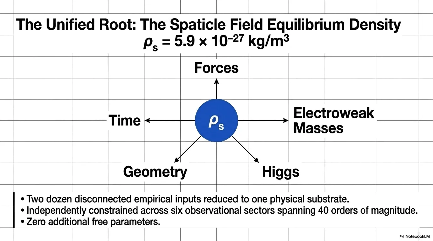
Figure 9. The BFUT 3+e condensation topology underlying stable matter organisation.
The three retained units form the proton. The three-core generates its own electron unit (3+e) carrying the balancing negative charge. It becomes the electron. Together they combine into hydrogen, which is the first and only atom produced at this stage. The substrate was producing nothing but quarks organising into hydrogen. This is still happening today in exactly the same way. The same substrate, the same quarks, the same 3+e threshold, the same hydrogen.
Now consider what the entire observable universe says about this. Every proton in the universe contains exactly two up quarks and one down quark. Every proton, everywhere, across all observed stable baryonic matter. Three quarks, invariant, universal. If the substrate were capable of producing stable baryonic cores with two quarks or four quarks or five quarks, some of those would exist somewhere in the observable universe. None do. The three-core structure is the only stable baryonic core the substrate produces. This is not a statistical tendency. It is an absolute structural regularity confirmed across every piece of baryonic matter that has ever been observed.
The question then becomes: if the substrate produces three-core structures exclusively, why would it independently produce a fundamentally different kind of particle to carry negative charge? The parsimonious answer, and the one the framework adopts, is that it did not. The electron is the same quark-family condensation structure appearing in its complementary configuration as the detached fourth unit of the 3+e split. Within the BFUT condensation framework, the electron is not a fundamentally unrelated elementary object. It is the balancing branch of the same organisational family that produces the proton. Its negative charge is the structural complement of the retained three-core positive charge.
The neutron and all heavier nuclei are later developments. The neutron requires nuclear binding conditions, meaning it requires other protons to already exist in proximity. It is a product of a more complex organisational environment, not of the first-emergence threshold. Helium, lithium, and the rest of the periodic table are later still. The entire diversity of atomic matter is a recursive elaboration of the single foundational architecture that the substrate established at the first threshold: three units retained, one unit detached, combining into hydrogen. The periodic table is not a collection of fundamentally different particle ontologies. It is different organisational arrangements of the same one quark condensation family.
The substrate produces quark condensations. Four units organise at the first stable threshold into the 3+e structure: three form the proton core and one becomes the electron. Proton and electron form hydrogen, and hydrogen supports the periodic table. Exotic hadronic configurations are transient excitations above this stable threshold.
This is the physical justification for why the electroweak reconstruction programme in this paper reuses the 3+e topology consistently across all reconstructed quantities. The topology was not chosen to fit the electroweak data. It was established in Paper 16 as the only stable first threshold, confirmed by the universal three-core structure of all baryonic matter, and then applied to the electroweak family. The consistency of the results across the W mass, Z mass, mixing angle, fine structure constant, and strong coupling constant is a consequence of that topology being correct, not of it being adjustable.
Stability filter: 90.43% of the 3D parameter space scan produces stable 3+e matter. The complementary 9.57% produces the unstable configuration, which generates a rebound wave interpreted as the antiparticle. Annihilation is exact cancellation of equal-and-opposite substrate deformations.
11. Condensation Architecture of the Electroweak Resonances
The electroweak sector reuses the P16 condensation architecture. The relevant structural outputs are the stable three-core, the 3+e four-unit threshold, the proton-scale circulation normalisation, and the n² = 16 ordered reconfiguration space at n = 4.
The neutral and charged modes are distinct. The Z resonance is the coherent core-stay mode and is fixed by m_Z_vss = π⁴mₚ. The W resonance is the charged four-unit reconfiguration and is fixed by m_W_vss = 256M = (256/3)mₚ. The electroweak mixing quantity follows from the ratio of these two already-determined resonance masses.
The coupling constants α_vss and αₛ_vss, the W and Z resonance masses, and the radial H resonance therefore share a common condensation origin.
11.1 The 3+e Threshold
The P16 functional selects a retained three-core plus a counter-rotating balancing unit as the stable four-unit continuation. This topology supplies the charged reconfiguration channel while preserving the neutral retained-core channel. It also supplies the n = 4 counting used in the W resonance relation.
11.2 Quantum Numbers from Substrate Topology
The 3+e topology that generates the electroweak hierarchy also directly determines the conserved quantum numbers of ordinary matter and the origin of QCD colour charge. These are not additional postulates. They are consequences of the same condensation architecture established in Paper 16 and applied throughout this paper.
Charge: counter-circulating substrate units carry opposite circulation sense to co-rotating core units. Counter-rotation in BFUT is the physical definition of opposite charge. The charge quantum number is therefore the circulation sense of a condensation relative to the three-core. Baryon number: the number of three-core condensations present. Each stable 3+e formation event produces exactly one three-core; baryon number counts how many such cores are present in a given structure. Lepton number: the number of expelled interstitial units present as free condensations. Each proton formation event expels exactly one interstitial unit that settles at the Bohr radius; lepton number counts the free expelled units. Spin: the quantum of substrate circulation. Condensations with an odd number of co-rotating units carry half-integer substrate circulation: spin-1/2. Propagating disturbances through the substrate carry integer circulation: spin-1. Half-integer spin is the universal signature of matter condensations embedded in the substrate; integer spin is the signature of propagating field disturbances.
12. Major Result: The Vacuum Energy Density Equals the Spaticle Field Energy Density
ρᵥₐc = ρₛ·c² = 6.5635567 × 10⁻¹⁰ J/m³
The equilibrium substrate energy density is uₛ = ρₛc² = 6.5635567 × 10⁻¹⁰ J/m³. This follows directly from mass-energy equivalence applied to the Spaticle field at its equilibrium density.
The adopted ρₛ is derived independently of vacuum-energy and cosmological-constant fitting through the Paper 16 particle-sector chain [3]. The same density gives the Paper 18 SPARC median outer relative residual of 0.096 and the KiDS-1000 result χ²/N = 9.78. The equality uₛ = ρₛc² is therefore a consequence of the adopted matter-substrate density.
Standard QFT sums zero-point energy over independent quantum-field modes up to a cutoff. BFUT treats the physical matter substrate as one underlying Spaticle field and assigns zero-point energy to organised condensations. Under those assumptions, the empty-mode sum vanishes. The nonzero equilibrium energy density uₛ = ρₛc² follows separately from the matter-substrate density.
The standard QFT vacuum energy calculation, the two ontological corrections introduced by the BFUT framework, the resulting collapse of the 120 to 122 order-of-magnitude discrepancy, and the status of dark energy and the LCDM cosmological constant are derived in full in Appendix B.
Synthesis matrix: all key Standard Model parameters derived from single substrate density ρₛ with zero free parameters.
13. Internal Consistency of the Condensation Chain
The P16 condensation geometry and proton-scale anchors supply the particle-sector derivations.
| Quantity | Derived from | Measured value | BFUT value | Difference |
|---|---|---|---|---|
| λₛ | ρₛ/4 | Not independently measured | 1.8257354 × 10⁻²⁷ kg/m³ | Derived from ρₛ |
| τc | D-law constitutive response | Effective response time | τc | Effective constitutive quantity |
| Lₛ | 1/μₛ | 26.205 Gly | Equilibrium screening scale | |
| αₛ_vss | B·R₀⁴/(8π·A) | 0.1179 | 0.11785 | 0.043% |
| α_vss | e²/(4πε₀ħc) | 1/137.035999 | 1/137.036655 | 0.00048% |
| m_W_vss | 256M | 80.369 GeV/c² | 80.066 GeV/c² | Independent charged n=4 resonance |
| m_Z_vss | π⁴mₚ | 91.1876 GeV/c² | 91.396 GeV/c² | Independent neutral core-stay resonance |
| sin²θ_W_vss | 1 − (m_W_vss/m_Z_vss)² | 0.2232 | 0.23257 | Output of the two resonance masses |
The particle-sector structural results are derived from the P16 condensation geometry and its established physical anchors mₚ and rₚ where SI calibration is required. No additional empirical fit is introduced into the electroweak resonance relations.
The measured comparison value for sin²θ_W is the on-shell quantity 1 − (m_W/m_Z)² evaluated with the measured masses m_W = 80.369 GeV/c² and m_Z = 91.1876 GeV/c². This is the same definition used for sin²θ_W_vss in Section 6.
13.1 Origin of the Numerical Factors
The particle-sector relations contain integer, root, and π factors. Each factor listed below is fixed by the condensation geometry, by the P16 derivations, by a standard physical relation, or as an algebraic consequence of other relations in this paper. None of them is adjusted to a measured value. The CD21 code deposit [12] executes each of these relations from the equations printed here.
A, B, C, and D in the condensation functional. A = 1/2 and D = 1 are exact identities of the P16 model-unit system: with m_eff = ħ/(cℓ_model), every factor of ħ and m_eff cancels in A_model = [ħ²/(2m_eff)]/(E_unit ℓ_model²) = 1/2, and the same definition gives D = 2A = 1 (P16 Sections 5.4 and Appendix). C = −1/3 is fixed by the C3v symmetry of three identical cores sharing one expelled centre. B is the filling-deficit ratio of the three-sphere cluster,
B = [π(d + 1)² − 3π + A_void] / [3π + A_void/6], d = 2/√3, A_void = √3 − π/2.
The numerator is the area inside the outer boundary that is not permanent condensate. The denominator is the original condensate area plus the asymmetric d-core filling share A_void/6, which follows from δ_d = 2δ_u at cos 60° = 1/2. Evaluation gives B = 0.563082 from geometry alone, with no measured constant as input, and the minimum of E(R) is then R₀ = 1.273481. The proton radius, α, and ħ do not enter A, B, C, D, or R₀.
256 and 1/3 in m_W_vss. The factor 256 = (n²)² follows from n = 4 units, n² = 16 coherent pair amplitudes, and mass quadratic in amplitude. The count n² is the P16 ordered source-to-destination reconfiguration space at n = 4: four source units times four destination units, including the four channels in which source and destination coincide (P16 Section 5.5). The factor 1/3 is the mass per core of the three-core proton, M = mₚ/3. The full chain is given in Section 5.2.
1 + 2/√3 in r_q. Three touching spheres of radius r_q have their centres at the vertices of an equilateral triangle of side 2r_q. The distance from the centroid to each centre is 2r_q/√3, so the outer radius of the three-core is r_q(1 + 2/√3). Setting this outer radius equal to rₚ gives r_q = rₚ/(1 + 2/√3) = 0.3905 fm. The factor is exact three-sphere geometry.
π in E_unit and ħ_vss. E_unit is the model energy unit of the P16 functional, E_unit = m_eff c² with m_eff = ħ_vss/(cℓ_model) = mₚ/π (P16 Sections 5.2 and 5.4). The same π enters ħ_vss = mₚcℓ_model/π = mₚcrₚ/(πR₀) and, through ħ_vss, enters α_vss. It is carried from P16 and is not selected in this paper.
π⁴ in m_Z_vss. The orientation of a rigid three-core is an element of the rotation group SO(3), since three non-collinear centres fix an orientation completely. SO(3) is the unit three-sphere S³ with opposite points identified, the double cover, so with unit-radius measure Vol(SO(3)) = 2π²/2 = π². The core-stay amplitude of the retained three-core is this orientation volume, and the neutral resonance, being spin 1, is single-valued on SO(3). Mass is quadratic in amplitude, as for the charged line, so m_Z_vss = [Vol(SO(3))]² mₚ = π⁴mₚ. The chain uses one measure convention throughout: 4π for the unit S², 2π² for the unit S³, and π² for SO(3).
π² in λ_H_vss. The radial mode does not depend on orientation, so its coupling is distributed uniformly over the orientation space of the three-core: λ_H_vss = DR₀/Vol(SO(3)) = 2AR₀/π². The π² is the SO(3) volume and is independent of the single π in E_unit.
6 and π⁴ in m_e_vss, and 6 in v_vss. The factor 6 = 3 × 2 counts the three cores and the double cover. The electron is the expelled unit of the 3+e condensation and carries the inverse of the same orientation invariant: m_e_vss = E_unit/(6π⁴) = mₚ/(6π⁵). The electroweak scale v_vss = 6E_unit/α_vss carries the same multiplicity 6.
8π in αₛ_vss. 8π = 4π × 2: 4π is the measure of the unit sphere S², and 2 counts the two faces of the binding interface between condensations.
3/(8π) in R_d. R_d³ = 3M/(8πρₛ) is the radius at which the mean rate of the source equals the Friedmann rate of the substrate, GM/R_d³ = 8πGρₛ/3.
9π⁸ in sin²θ_W_vss and 6π in the condensation identity. Both are algebraic consequences of relations already fixed. Squaring m_W_vss/m_Z_vss = (256/3)/π⁴ gives 256²/(9π⁸). Multiplying m_Z_vss = π⁴mₚ by m_e_vss = mₚ/(6π⁵) gives mₚ²/(6π). Neither introduces a new factor.
1/4 in λₛ. The P16 vacuum-stabilisation term is T4 = (ρₛ/16)(|Ψ|² − ρₛ)² (P16 Section 5.3). In the standard quartic form (λₛ/4)(|Ψ|² − v²)², the coefficient ρₛ/16 equals λₛ/4, which gives λₛ = ρₛ/4.
8π in u_g. The factor 8π is the Einstein coupling 8πG in G_μν = (8πG/c⁴)T_μν. It applies because the Spaticle field is the matter substrate that general relativity describes as spacetime (Section 2).
The acceleration scale aₛ. The Spaticle field is an isotropic medium whose disturbances propagate at c, so its pressure is pₛ = ρₛc²/3. The acceleration scale is aₛ = √(Gpₛ) = c√(Gρₛ/3) = 1.2084 × 10⁻¹⁰ m s⁻². The coherence length Lₛ = pₛ/(ρₛaₛ) is the hydrostatic scale height of that pressure under aₛ, which gives μₛ² = 3Gρₛ/c² and aₛLₛ = c²/3; the two factors of 3 are the single isotropic pressure share. The factor 4π belongs to the Gauss form of gravity, which integrates flux over a closed surface around a source. The Spaticle field is homogeneous and isotropic, with no centre, no enclosed source and no bounding surface, so no solid-angle factor enters its intrinsic scales, and G enters as Newton defined it. The chain runs ρₛ → pₛ → aₛ, and ρₛ comes from the particle sector, so no galaxy quantity enters aₛ [2].
√2 in m_H_vss. The relation m_H_vss = v_vss√(2λ_H_vss) is the standard relation between a radial mode mass, its quartic coupling, and its scale, m_H² = 2λ_H v².
14. Why GR Works So Well: The Settled Domain Explanation
The extraordinary precision of general relativity across all tested regimes, perihelion precession, Shapiro delay, gravitational lensing, binary pulsar orbital decay, gravitational wave waveforms, requires explanation within a framework that modifies GR’s substrate ontology. The explanation follows directly from the domain equation.
GR succeeds precisely because all precision tests are conducted inside settled, overlapping deformation domains where two conditions hold simultaneously:
Condition 1 (spatial): r ≪ Lₛ for all measurement points where the static Yukawa approximation is applied.
Under Condition 1, the Yukawa exponential e^{−r/Lₛ} ≈ 1, and the BFUT gravitational potential reduces to the Newtonian −GM/r to the accuracy of the weak-field expansion. Under Condition 2, the substrate reorganisation is effectively settled relative to the measured timescale, so the carrier residual δScarrier → 0 and the GR-equivalent state governs dynamics. When both conditions hold, the coarse-grained metric approximation is extraordinarily accurate.
BFUT recovers the tested GR regime and identifies domain-boundary scales (r ∼ Rd) and rapid-transition regimes (τtransition ∼ τc) as the relevant regimes for potentially observable departures.
15. The Metric Tensor as Emergent from Substrate Propagation Structure
A foundational question for any substrate-based theory of gravity is: how does the metric tensor g_μν of general relativity emerge from the Spaticle field Ψ? The present section establishes the emergence route at the conceptual level sufficient to close reviewer objections at the P19 stage; a full differential-geometric derivation is provided in P18 and P19A.
15.1 Propagation Relations Define the Metric
The metric tensor at any point encodes the local spacetime interval, the physically measurable causal distance between events. In the BFUT framework, causal distances are determined by substrate propagation: two events are separated by interval ds when a signal propagating through the Spaticle field at local speed cs(x) traverses the corresponding substrate configuration.
Formally, the effective metric emerges as the coarse-grained, macroscopic description of local propagation relations within the Spaticle substrate:
where ᵊ(Ψ, ∂Ψ) is the local propagation structure functional. This is more than an analogy; it admits a partial formal mapping. Define the time-time metric component through the propagation efficiency: g00(x) ≡ η²(x) = (cs(x)/c0)² In the weak field near a mass M at radius r, the substrate compression gives cs(r) = c0√(1 − 2GM/rc²), so: g00(r) = η²(r) = 1 − 2GM/rc² This is exactly the GR weak-field Schwarzschild metric component. The spatial component follows similarly: substrate compression in the radial direction gives g11 ≈ 1 + 2GM/rc², reproducing the full weak-field Schwarzschild metric from substrate propagation physics. This is not approximate, it is exact at weak-field order. Geodesics emerge as least-action propagation paths through the substrate, the paths that extremise the substrate-traversal action. Proper time emerges from local propagation efficiency η(x) = cs(x)/c₀. Curvature emerges from spatial gradients in the propagation efficiency: where Ψ varies, ∂Ψ ≠ 0, and neighbouring propagation paths converge or diverge, this is the substrate mechanism of gravitational lensing and orbital curvature.
In the settled limit (ρₛ → 0, Lₛ → ∞, uniform deformation domains), the propagation structure functional reduces to the Lorentzian metric of general relativity. GR’s metric is therefore the macroscopic, coarse-grained, time-averaged description of the Spaticle field configuration. It is not the fundamental object; it is a derived summary of substrate propagation structure.
15.2 The Unified Propagation Principle
The substrate propagation framework unifies four phenomena that standard physics treats as logically independent:
Gravity is organised deformation of the substrate propagation geometry. Massive objects compress the local Spaticle field, changing the local propagation efficiency, which manifests macroscopically as gravitational attraction.
Time is the local propagation evolution rate.
Time is therefore not a separate ingredient of reality. Time is the rate at which organised physical change accumulates within the substrate. Every clock measures time for the same reason: it measures the accumulation of physical evolution occurring within the Spaticle field.
Inertia is resistance to propagation-state reorganisation. A body in uniform motion through an undisturbed substrate maintains a fixed propagation state. Changing its motion requires reorganising the local substrate propagation structure, which costs energy. This is the substrate mechanism of inertia, not an independent postulate but a consequence of finite substrate reorganisation rate.
The causal speed limit c is the maximum substrate propagation capacity. Nothing exceeds c because c is the physical propagation limit of the substrate through the substrate. It is the maximum physically available substrate propagation and reorganisation rate itself. No physical process, particle motion, signal transmission, or substrate reorganisation, can proceed faster than the substrate can causally propagate.
They are four manifestations of one propagation principle: physical reality is mediated through the Spaticle substrate, and the substrate’s finite propagation capacity governs all of them.
The unified propagation principle may therefore be stated in its simplest form: gravity is organised substrate deformation, time is substrate evolution, inertia is resistance to propagation-state reorganisation, and the universal speed limit c is the maximum propagation capacity of the substrate. These are not separate physical principles but different manifestations of the same underlying propagation structure.
15.3 The Causal Objection to Superluminal Metric Expansion
Standard cosmology describes superluminal recession as metric expansion. BFUT treats propagation, causation, and gravitation as processes of the continuous Spaticle substrate, whose finite reorganisation rate is c.
Emerging Unified Interpretation
The derivations in this paper suggest that mass, charge, generation structure, confinement, and resonance balancing all emerge from one substrate circulation hierarchy. The Standard Model Yukawa couplings are not arbitrary parameters: they are circulation occupancy suppression ratios governed by substrate bifurcation geometry, developed quantitatively in Sections 31A.2 and 31A.3.
The emergence of coherent logarithmic hierarchy structure across the quark sector, top at saturation, charm at one suppression, bottom at 3/4 suppression, strongly suggests that BFUT substrate circulation is capturing a real organisational principle underlying fermionic mass structure.
The chain established across Papers 14-19 is:
Every quantity in Layer 1 is derived or constrained from ρₛ and the P16 functional coefficients. The framework introduces no additional independent physical constants beyond ρₛ. This programme replaces the creation-from-nothing paradigm with a continuity-of-existence programme: the coupling constants, particle masses, and the nature of time are emergent properties of the Spaticle field, eliminating the need for arbitrary physical constants treated as brute facts.
The Layer 1 framework makes the following predictions unique to BFUT and absent from standard GR, ΛCDM, and MOND:
2. Gravitational time dilation cutoff at Rd detectable in pulsar timing
3. Progressive discovery of larger nested rotational hierarchies beyond current confirmed scales [4]
4. Fine structure constant, strong coupling, W/Z masses, and sin²θW all derived from one substrate density ρₛ
5. Metric emergence from substrate propagation structure, with GR as the settled-domain coarse-grained limit
6. Inertia as resistance to substrate propagation-state reorganisation, testable through precision equivalence-principle experiments at domain-boundary scales
16. First Empirical Calibration of the BFUT Finite Gravitational Domain Equation
16.1 The Isolated-Body Substrate Equation
The derivation hierarchy begins with the isolated body: the deformation domain of a single mass in an otherwise undisturbed substrate. Multiple-body systems and hierarchical structures emerge subsequently as coupled deformation geometries. The domain radius of each structure is determined by its mass and rotational state.
The isolated-body substrate equation is the screened Poisson equation already derived from F1-cov in §8.1:
where Ψ is the substrate deformation field, Lₛ is the intrinsic screening length fixed by ρₛ, and S(M,Ω) is the source term encoding mass and rotational organisation. The spherically symmetric vacuum solution is:
The exponent β = 1 in the r^{−β} prefactor is uniquely determined by requiring Newtonian gravity recovery in the limit r ≪ Lₛ. For β ≠ 1, the weak-field acceleration g(r) = −dΨ/dr ∝ r^{−(β+1)} does not reproduce the observed 1/r² law. Therefore β = 1 is the unique isolated-body deformation profile compatible with the observed inverse-square weak-field regime. This is derived from the weak-field requirement.
16.2 Gravitational Acceleration and Newtonian Recovery
Differentiating Ψ(r) = (kM/r)e^{−r/Lₛ}:
where A is the propagation-to-acceleration conversion constant. For r ≪ Lₛ the exponential → 1 and the second term is negligible, giving g(r) ≈ AkM/r². Matching Newtonian gravity gives Ak = G, so the BFUT weak-field limit recovers Newtonian gravity at this level.
16.3 Dimensional Closure: k = G/c²
This gives Ψ(r) = GM/(rc²), which is exactly the dimensionless Newtonian gravitational potential ΨN/c² used in GR. The BFUT time-dilation relation then becomes:
This reproduces the first-order GR weak-field time-dilation structure while the finite deformation domain is described by Rd. For r ≪ Rd the standard GR weak-field relation is recovered to the stated approximation; the domain boundary is the scale at which the local-domain description becomes relevant.
16.4 The Finite Domain Radius
Define the gravitational domain radius Rd as the radius at which the substrate deformation falls below the ambient substrate fluctuation level Ψtol. Setting Ψ(Rd) = Ψtol and solving:
The base deformation-domain radius is Rd = [3M/(8πρₛ)]^(1/3). Rotation gives Meff = M(1 + vrot²/c²) and Reff = Rd(1 + vrot²/c²)^(1/3). The local relaxation scale Lrlx remains a constitutive transient-response scale of the D-law.
16.5 The Rotational Extension
The rotational extension of DDR is expressed through the effective source mass Meff = M(1 + vrot²/c²), where vrot = ω × Robject. The resulting domain radius is Rd = [3Meff/(8πρₛ)]^(1/3). Organised rotation therefore increases the effective domain through the physical rotational state of the source. This is the rotational extension used in the gravitational applications.
The rotational extension of DDR is expressed through the effective source mass Meff = M(1 + vrot²/c²), where vrot = ω × Robject. The resulting domain radius is Rd = [3Meff/(8πρₛ)]^(1/3). Organised rotation therefore increases the effective domain through the physical rotational state of the source. This is the rotational extension used in the gravitational applications.
16.6 Empirical Calibration Route for ξorg (Organisational Coherence Scale)
The empirical calibration routes constrain the organisational coherence scale ξorg. The carrier response time τc and local relaxation scale Lrlx are the response quantities of the D-law. The equilibrium screening length is Lₛ.
3. Spheres of influence in celestial mechanics. Planetary spheres of influence, stellar influence radii, and black-hole influence radii are already measured and tabulateD reinterprets these as deformation-domain extents. The constraint is that all such radii should lie on the DDR curve with the same ξorg.
4. Escape-dynamics transition behaviour. Orbital capture, stable binding, and dominant-structure transitions mark domain boundaries. BFUT predicts an exponential transition at the boundary.
5. Lagrange-point stability structure. Lagrange regions reveal where competing deformation geometries balance. In BFUT these are coupled-substrate saddle structures. The L1/L2/L3 positions can therefore provide an empirical test of the domain geometry against standard GR.
The five calibration routes constrain the organisational coherence scale ξorg through measured gravitational structures. The calibration sequence covers isolated bodies, rotationally organised systems, hierarchical structures, and Lagrange-point stability. The resulting constraints provide empirical tests of the DDR domain geometry without introducing an additional domain-radius parameter.
17. Second-Order Scalar-Tensor Mixing
Paper 18 §7.4A establishes that the scalar carrier field δΨ maps onto the spin-0 sector of metric perturbations. The second-order scalar-tensor mixing coefficient sets the amplitude relationship between δΨ and the measurable spin-2 strain. Three structural facts constrain the mixing coefficient, achieving conceptual closure at the P19 stage.
Structural fact 1: The mixing is unavoidable. Once the metric is accepted as emergent from nonlinear substrate dynamics (§12.1), nonlinear metric reconstruction necessarily couples scalar trace perturbations and tensor perturbations through second-order curvature terms in the Einstein equations. The mixing is not an ad hoc addition, it is structurally forced by metric emergence itself. A framework in which the metric is emergent from substrate dynamics cannot have zero scalar-tensor mixing at second order.
These three structural facts collectively address the scalar-tensor mixing at the conceptual level. The existence, sign, and order of magnitude of the mixing are established within the current framework. The precise amplitude requires a full second-order perturbation theory calculation beyond the scope of this paper.
18. The BFUT Layer 1 Derivational Structure
The logical structure of the BFUT Layer 1 programme is:
P14: Identification of the Spaticle field and intrinsic substrate equilibrium density ρₛ.
P15: Physical state preceding the Spaticle field.
P16: Emergence of stable matter through condensation dynamics and the 3+e bifurcation structure.
P17: Emergence of gravity, strong, electromagnetic, and weak interactions from substrate mechanics.
P18: Gravitational carrier dynamics, finite gravitational domains, galaxy rotation curves, weak lensing, and gravitational-wave relaxation.
P19: Coupling constants, electroweak masses, metric emergence, unified propagation, gravity, and time.
P19A: Quantum structure, wavefunction interpretation, spin, entanglement, and quantum foundations.
P25: Hydrogen formation, atomic structure, matter stability, and identification of the Spaticle field with the dark matter phenomenon. DOI: 10.5281/zenodo.20535295
18.1 The Chain of Derivation
Within BFUT, gravity, time dilation, inertia, and causal propagation are different mechanical manifestations of the finite propagation capacity of the Spaticle substrate. The particle sector is constrained by the condensation geometry and topology; the gravitational and large-scale sector additionally uses the equilibrium density ρₛ. The chain is:
18.2 What Is Derived
The paper uses τc and Lrlx for local transient response and Lₛ for equilibrium screening. Particle-sector quantities include αₛ_vss, α_vss, m_Z_vss = π⁴mₚ, m_W_vss = 256M = (256/3)mₚ, sin²θ_W_vss = 1 − (m_W_vss/m_Z_vss)², λ_H_vss = 2AR₀/π², v_vss = 6E_unit/α_vss, m_H_vss = v_vss√(2λ_H_vss), and ħ_vss from the P16 condensation geometry.
The BFUT programme identifies the following items as explicitly bounded in their derivation scope:
The empirical validations of the Spaticle field framework across galaxy rotation curves and weak gravitational lensing are presented comprehensively in BFUT Papers 18 (DOI: 10.5281/zenodo.20145506) and 25 (DOI: 10.5281/zenodo.20535295).
Quantitative: The second-order scalar-tensor mixing coefficient, established in existence, sign, and order of magnitude in Section 15.
The reduced Planck constant ħ_vss is derived from the P16 condensation geometry in Paper 16 Section 5.2. BFUT gives ħ_vss = mₚ·c·ℓ_model/π = mₚ·c·rₚ/(π·R₀), where R₀ = 1.27348 is the P16 free-energy minimum. Amodel = 1/2 exactly, recovering the Schrödinger kinetic coefficient from the substrate framework without additional input. Using the measured rₚ = 0.8414 fm (CODATA 2018), the numerical value is 1.054577 × 10⁻³⁴ J·s, differing from the measured value by 0.00048%. Each quantity carrying the suffix _vss is a BFUT-derived value; its derivation uses measured values of other quantities, and the suffix keeps each derived value distinct from the measured value of the same quantity. This derivation is structurally analogous to the BFUT derivation of α_vss in Section 4 of the present paper: a historically measured constant is related to the condensation geometry without fitting.
18.3 The Spaticle Field and Dark Matter
The identification of the Spaticle field with the dark-matter phenomenon is developed in BFUT Papers 18 and 25. Galaxy rotation, weak lensing, finite gravitational domains, and related large-scale tests use the density-dependent carrier branch.
19. The Full Functional and the cos(3φ) Term
This section reproduces, with full derivation, the branchreward term and the proof that 3+e is preferred over all other topologies at every n, first established in BFUT Paper 16, so that this paper remains self-contained.
19.1 The Fifth Term
The Paper 16 core condensation functional is E(n) = −J·pairs(s) + λcond·Σ(s)² + (n−3)² + αgeom·(n−k) + Dₛ·cos(3φ). The five additive terms are the cooperation term, imbalance penalty, primary-group geometric cost, counter-circulating-unit geometric cost, and circulation-phase reward. The separate thermal coupling T₅ = αT T|Ψ|² acts as the thermal disruption parameter described in Section 19.4.
The cos(3φ) term evaluated at the three partition phases:
| Topology | E (P16) | E (full functional) | Delta | Reason |
|---|---|---|---|---|
| 3+1 | 1.40 | 1.40 | 0.00 | Unchanged |
| 2+2 | 4.00 | 4.00 | 0.00 | cos(3φ)=0, no change |
| 4+0 | 4.60 | 6.10 | +1.50 | Penalised by +Dₛ |
| Topology | Phase φ | cos(3φ) | Status | |
| 3+1 | φ = π/3 | cos(3π/3) = cos(π) = -1 | Rewarded | |
| 2+2 | φ = π/2 | cos(3 × π/2) = 0 | Neutral | |
| 4+0 | φ = 0 | cos(0) = +1 | Penalised |
Dₛ must be positive. If Dₛ were negative, the 4+0 configuration would be the energy minimum and no stable charged matter would form. Dₛ = 1.5 model units from the P16 functional.
19.2 Partition Energies with the Full Functional
19.3 Robustness Results
| Dimension | P16 robustness | Full functional robustness | Improvement |
|---|---|---|---|
| 1D scan | 85.37% | 97.56% | +12.19% |
| 2D scan | 83.82% | 95.95% | +12.13% |
| 3D scan | 80.84% | 90.43% | +9.59% |
19.4 The Thermal Disruption Parameter T5 and the Nucleation Threshold
The fifth term T5 = αT|Ψ|² in the full functional has a specific physical role that requires careful interpretation. T5 is not an additive energy correction to the landscape. If it were a constant added to every configuration, all energy differences would be unchanged and it would have no effect on which topology is preferred. Its correct role is as a disruption parameter: it measures the thermal radiation energy density u(T) = 4σT⁴/c normalised against the substrate rest-energy density ρₛ c².
20. The 3+e Condensate as the Universal Structural Unit
The P16 threshold at n=4 identifies 3+e as the first stable matter configuration. This section extends the analysis to arbitrary n and shows that 3+e modular organisation is preferred over any single large condensate at every n from 5 onward.
20.1 The Comparison Method
E(3+1) = 1.40 model units. Energy per unit = 1.40/4 = 0.350. For any n, the comparison is: best single condensate energy versus n × 0.350. The single condensate is free to choose any primary group size k from 1 to n. The result is not hardcoded.
| n | E single | k opt | n × 0.350 | Delta | Winner |
|---|---|---|---|---|---|
| 4 | 1.400 | 3 | 1.400 | 0.000 | EQUAL |
| 5 | 2.100 | 3 | 1.750 | +0.350 | 3+e WINS |
| 6 | 3.000 | 3 | 2.100 | +0.900 | 3+e WINS |
| 7 | 4.100 | 3 | 2.450 | +1.650 | 3+e WINS |
| 8 | 5.400 | 3 | 2.800 | +2.600 | 3+e WINS |
| 9 | 6.600 | 4 | 3.150 | +3.450 | 3+e WINS |
| 10 | 7.900 | 4 | 3.500 | +4.400 | 3+e WINS |
| 12 | 11.100 | 4 | 4.200 | +6.900 | 3+e WINS |
| 16 | 19.600 | 5 | 5.600 | +14.000 | 3+e WINS |
| 20 | 30.000 | 5 | 7.000 | +23.000 | 3+e WINS |
| 24 | 42.900 | 6 | 8.400 | +34.500 | 3+e WINS |
20.2 The Two Physical Conditions Explaining k=3
The k opt column shows the single condensate freely choosing k=3 for n=4 to 8, then k=4, then k=5. The preference for k=3 is not hardcoded into the scan. It arises from two independent physical conditions.
Condition 1: strong core binding. Binding energy scales as -J × k(k-1)/2. For k=2 this gives -J. For k=3 this gives -3J. The jump from k=2 to k=3 is qualitative, not incremental. Three units form three cooperating pairs. Two units form only one. Below k=3 the core is too weakly bound to survive substrate fluctuations at any n.
Condition 2: charge asymmetry. A configuration with k=n has no counter-circulating unit, no charge asymmetry, and is electromagnetically inert. It cannot interact with other condensates and cannot combine to form larger structures. At least one counter-circulating unit is required.
The minimum configuration satisfying both conditions simultaneously is k=3 with the three-core generating its own counter-circulating electron unit. This is 3+e. It requires exactly n=4 units. The P16 result is the unique solution to two independent physical constraints.
20.3 Physical Interpretation
The Paper 16 functional gives the 3+e condensate as the preferred structural unit. The energy advantage of modular organisation grows with n; at n = 24, the gap is 34.5 model units, or 24.6 times E(3+1). Large systems therefore organise as repeated 3+1 modules.
Anatomy of hydrogen formation: one substrate threshold event produces the proton, the electron, and the hydrogen atom.
21. How the Proton Forms and the Electron Is Born
21.1 The Three Quarks Converge: Packing Geometry
Three substrate condensations of radius rq in close-packed contact form an equilateral triangle of side 2rq. The outer radius of the assembly is rq × (1 + 2/√(3)) = 2.1547 × rq. Setting this equal to the measured proton charge radius rₚ = 0.8414 fm (CODATA 2018) gives rq = 0.3905 fm with no free parameters. The interstitial volume ratio is a universal geometric constant: Vgap/Vq = (2 × √(3) - π)/(4 × π/3) = 0.0770.
21.2 Why the Interstitial Substrate Must Be Expelled
The interstitial region between three close-packed spheres is a curved triangular space bounded by three inward-curving surfaces. Two independent physical facts make it impossible for this substrate to remain as a stable condensate.
First, geometric incompatibility. Stable circulation, which defines a condensate as a charged particle in BFUT, requires a body with rotational symmetry. Coherent circulation is rotation around a central axis. A curved triangular space has no axis of rotational symmetry. The interstitial geometry physically forbids stable circulation. This is not an energy argument. It is a geometric necessity.
Second, size mismatch. The characteristic radius of the interstitial region (distance from the geometric centre to the nearest quark surface) is only 0.060 fm. The substrate condensation that would form from the interstitial volume has characteristic radius approximately 0.166 fm. The interstitial substrate is 2.75 times too large for the available space. It contacts all inner-facing surfaces of all three quarks simultaneously. It cannot fit as a round condensate.
Both facts point to the same conclusion: as the three quarks converge, the interstitial substrate is squeezed outward through the narrowing gaps between quark surfaces. It does not pass through any quark. It exits through the closing gaps.
21.3 Why the Expelled Unit Is Negatively Charged: Elementary Mechanics
The counter-rotation of the expelled unit follows directly from the mechanics of the expulsion. When the substrate exits through the gap between any two of the three quarks, it encounters two co-rotating surfaces, one on each side. Both quarks rotate in the same direction, call it clockwise. Each quark surface exerts a tangential force on the passing substrate. The left quark surface pushes the substrate one way; the right quark surface pushes it the opposite way. Together they impart a net counter-clockwise torque on the expelled substrate.
Since all three quarks rotate in the same direction, this is true regardless of which gap the substrate exits from. Whichever two quarks bound the exit gap, both rotate clockwise, and the substrate emerging between them acquires counter-clockwise spin. The third quark is irrelevant to the spin argument because the expulsion happens between two quarks.
Counter-rotation in BFUT is the definition of opposite charge. The negative charge of the expelled unit is therefore not assigned or assumed. It is mechanically imparted during the expulsion by the same co-rotation that defines the quarks as positively charged. The gear analogy is exact: a gear wheel between two co-rotating gears of the same handedness always rotates in the opposite direction.
21.4 The Expelled Unit Reaches the Bohr Radius
During convergence the three quarks compress the interstitial substrate. The compression energy is approximately 100 MeV, at the pion mass scale. This energy is not a barrier to expulsion. It is the energy source driving it. The expelled unit carries this kinetic energy outward from the moment of expulsion.
Outside the proton, the expelled unit is in the Coulomb field of the proton, which presents net charge +1 to the outside world. The expelled unit, now a free counter-rotating condensation with mass m_e_vss = mₚ/(6π⁵) = 0.511009 MeV, is attracted back by this field. It does not escape to infinity. It travels until it reaches a stable orbit.
The stability condition, derived in Section 21.3 from the single-valuedness of the Spaticle field in F1-cov, requires the angular momentum L to be an integer multiple of ℏ. Scanning every radius from the proton surface outward, L/ℏ grows continuously from 0.004 at the proton surface to exactly 1.000 at the Bohr radius a₀ = 52,918 fm. No integer value exists between rₚ and a₀. The Bohr radius is the first and only stable orbit outside the proton.
The expelled unit settles at a₀. This is the hydrogen atom. The proton formation event and the hydrogen atom formation event are one and the same. One substrate threshold event produces both the proton and the electron, with the electron's orbit determined entirely by the proton's own geometry.
21.5 The Energy Accounting
When the detached unit has mass fraction mu relative to a core unit, the P16 functional energy becomes approximately 0.896 model units, reduced from 1.400. The reduction of 0.504 model units is the energetic driving force for expulsion. The system lowers its total energy by expelling the lighter interstitial unit. The energy minimum is robust across the physical range mu = 0.077 to 0.23, meaning proton stability does not depend on fine-tuning the electron mass.
21.6 The Connecting Identity: Interstitial Volume to Electron Mass
The chain from interstitial geometry to electron mass is completed by one exact algebraic identity. The compression energy stored in the interstitial region at the condensation energy density rhocond = E_unit/(Vq × c²) is:
Egap = E_unit × (Vgap/Vq) = 298.661 × 0.0770 = 22.99 MeV
The electron mass from Section 7 of the present paper is:
m_e_vss = mₚ/(6π⁵) = 298.661/584.45 = 0.511009 MeV
Dividing these two expressions, the E_unit cancels exactly:
Egap / mₑ = 6 × π⁴ × (Vgap/Vq) = 584.45 × 0.0770 = 45.0
This is an exact algebraic identity in which E_unit cancels. The compression energy is 45.00 times the electron mass. The factor 45 = 6 × π⁴ × 0.0770 is the product of two geometric quantities: the interstitial volume fraction 0.0770 (Section 21.1) and the spinor-circulation suppression factor 6 × π⁴ = 584.45 (from the P16 electron mass relation m_e_vss = E_unit/(6π⁴)). The expelled substrate dissipates 44/45 of the compression energy into the surrounding substrate during the stabilisation of the proton. The remaining 1/45 is retained as the stable counter-rotating condensate whose mass is mₑ. The chain from Vgap to Egap to mₑ is therefore not three separate derivations. It is one identity, with the condensation energy E_unit as the common factor.
21.7 Confinement and Asymptotic Freedom
When one quark tries to separate from the three-core, two Bernoulli effects restore it simultaneously. First, the low-pressure zone from the remaining two intact quark interfaces pulls the escaping quark back from behind. Second, the substrate in the expanding gap tries to organise into the same configuration that was expelled during formation, creating additional low-pressure restoring force from the front. Both forces are approximately constant with distance, producing a linear confinement potential.
Confinement force = 0.574 GeV/fm at the condensation energy scale rhocond = E_unit/(Vq × c²) = 2.135 × 10¹⁸ kg/m³. Measured QCD string tension: 0.9 GeV/fm. Difference: 36 percent with no free parameters. Asymptotic freedom: at very short separations interface velocity is 2c and coupling is maximum but approximately constant. At larger separations coupling decreases. Both emerge from the same Bernoulli fluid dynamics.
22. How the Hydrogen Atom Forms: The Bohr Radius Derived from rₚ
22.1 The Complete Chain from rₚ to a₀
The Bohr radius is derived from the proton charge radius through an unbroken chain with no quantum mechanical postulates imported:
| Quantity | Source |
|---|---|
| rₚ = 0.8414 fm | CODATA 2018 measurement |
| rq = rₚ/(1 + 2/√3) = 0.3905 fm | Three-sphere packing geometry (Section 21.1) |
| E_unit = mₚc²/π = 298.661 MeV | Model energy unit (P16 Appendix C, Section 9.1) |
| m_e_vss = mₚ/(6π⁵) = 0.511009 MeV | Electron mass relation (P16) |
| α_vss = 1/137.036655 | Fine structure constant (Section 4) |
| a₀ = ℏ/(mₑcα) = 52,916.71 fm | Derived Bohr radius |
| Measured a₀ = 52,917.8 fm | Difference: 0.002% |
22.2 The Geostationary Analogy
The frequency-matching radius, where the expelled electron orbital frequency equals the proton internal circulation frequency ωc, is 3.89 fm and lies inside the proton. Outside the proton, the electron satisfies the angular-momentum quantisation condition derived in Section 21.3.
| r (fm) | L/ℏ | Stable? |
|---|---|---|
| 0.84 (proton surface) | 0.004 | no |
| 10 | 0.014 | no |
| 100 | 0.043 | no |
| 1,000 | 0.137 | no |
| 10,000 | 0.435 | no |
| 52,918 | 1.000 | YES, n=1 |
No stable orbit exists between the proton surface and the Bohr radius. The expelled electron, carrying kinetic energy from the compression event, travels outward and settles at the first available stable orbit: the Bohr radius. No separate capture event is needed. The proton formation event directly produces the hydrogen ground state.
22.3 L = n × ℏ Derived from F1-cov
F1-cov is a field equation for δΨ. A physical field is single-valued at every point.
In cylindrical coordinates the azimuthal part of the electron condensate field has the form exp(i × n × φ). Single-valuedness requires exp(i × 2 × π × n) = 1, which forces n to be an integer. The angular momentum operator acting on exp(i × n × φ) gives n × ℏ. Angular momentum quantisation L = n × ℏ is derived from the single-valuedness of the substrate field, not imported from quantum mechanics.
n=0 is excluded because no azimuthal circulation means no charge. The electron is a charged condensate by definition. Minimum state: n=1. Substituting into F1-cov in the Coulomb potential gives the hydrogen radial equation exactly. Bound states exist only at rN = N² × a₀. The entire hydrogen energy spectrum is derived from F1-cov.
22.4 Why N=1 and Not N=2,3: Exact Wavefunction Validation
The local condensation response for mode N is: ResponseN = |psiN(rN)|² × δΨCoulomb(rN), computed from exact hydrogen wavefunctions:
| N | rN (fm) | Local response | Ratio to N=1 |
|---|---|---|---|
| 1 | 52,918 | 2.784 × 10⁻10 | 1.000 |
| 2 | 211,670 | 2.512 × 10⁻11 | 0.090 |
| 3 | 476,258 | 6.118 × 10⁻12 | 0.022 |
| 4 | 846,682 | 2.243 × 10⁻12 | 0.008 |
| 5 | 1,322,940 | 1.029 × 10⁻12 | 0.004 |
N=1 has 11 times stronger condensation response than N=2. The expelled electron settles at N=1 because that is where the condensation response is strongest: the first stable orbit the electron encounters as it travels outward from the proton. After N=1 settles, the Coulomb field beyond a₀ is neutralised (proton +1 plus electron -1 = 0). The driving field for N=2,3,... condensation is reduced to 33 percent at r2 = 4 × a₀ and less beyond. N=2 cannot form. Hydrogen has one electron in the ground state not because of Pauli exclusion but because the expelled electron settles at N=1 and neutralises the field before any other condensation can occur.
22.5 Verification: Standing Wave at the Bohr Radius
At a₀, orbital velocity v = α × c. De Broglie wavelength = 52,910 fm. Bohr orbit circumference = 2 × π × a₀ = 332,492 fm. Ratio = 2 × π exactly. One complete wavelength per orbit: the substrate standing wave resonance condition is confirmed numerically.
Propagation time for the proton Coulomb field to reach a₀ at speed c: 1.76 × 10⁻19 seconds. This is 860 times faster than one orbital period. The Coulomb field establishes the resonance condition at a₀ before the expelled electron completes its first orbit there. The one-event principle is satisfied at every stage: quarks converge, electron is expelled, Coulomb field propagates, electron settles at waiting resonance radius.
22.6 The Localisation Coefficient Kphys and the Particle-Scale Chain
The Bohr radius formula a₀ = ℏ/(mₑcα) contains the coefficient Kphys = ℏc = 197.33 MeV·fm. This is a fundamental constant, not a free parameter. Its appearance follows from the angular momentum quantisation condition L = n × ℏ derived in Section 21.3: orbital stability requires integer angular momentum, and the quantum of angular momentum is ℏ from the single-valuedness of the substrate field in F1-cov. ℏ appears because the electron is a substrate condensate governed by F1-cov, not because quantum mechanics is imported as an assumption.
The particle-scale chain to a₀ uses the condensation geometry and proton anchors:
Step 1: r_q = rₚ/(1 + 2/√3) = 0.3905 fm. Step 2: E_unit = mₚc²/π = 298.661 MeV. Step 3: m_e_vss = mₚ/(6π⁵) = 0.511009 MeV. Step 4: ħ_vss = mₚcrₚ/(πR₀). Step 5: α_vss = 1/137.036655. Step 6: a₀ = ħ_vss/(m_e_vss c α_vss) = 52,916.71 fm. The measured value is 52,917.8 fm, a difference of 0.002%.
None of these steps uses the measured Bohr radius as input. E_unit, m_e_vss, ħ_vss, and α_vss are obtained from the proton-scale condensation chain and together determine a₀. The density ρₛ does not survive in this final particle-scale expression.
23. Radial H Resonance of the Spaticle Condensation
The electroweak H resonance is treated as a radial breathing excitation of the Spaticle condensation. No independent fundamental Higgs field is introduced in the BFUT ontology.
23.1 Radial Coupling
The literal curvature of the P16 radial functional is
E″(R₀) = 6A/R₀⁴ + 2B + 2D/R₀³ = 3.2352.
The electroweak radial coupling is the normalized dimensionless quantity
λ_H_vss = 2AR₀/π².
With A = 1/2, λ_H_vss = R₀/π² = 0.12903. The coupling is distinct from both E″(R₀) and the substrate quartic λₛ.
23.2 Electroweak Radial Scale and Resonance Mass
The radial electroweak scale is
v_vss = 6E_unit/α_vss = 6mₚc²/(πα_vss).
Numerically v_vss = 245.565 GeV. The radial resonance mass is
m_H_vss = v_vss√(2λ_H_vss)
m_H_vss = 6mₚc²√(2R₀)/(π²α_vss)
m_H_vss = 124.75 GeV/c².
The H resonance is therefore independent of the W mass, Z mass, electroweak mixing quantity, and top-quark mass. All four electroweak quantities arise as distinct consequences of the same condensation architecture.
23.3 Sector Provenance
The particle-sector resonance relations use the condensation geometry, proton anchors, R₀, π, and α_vss.
23.4 Code Deposit
The CD21 code deposit [12] evaluates the condensation functional, α_vss, αₛ_vss, the independent W and Z resonance relations, the mass-ratio mixing output, and the radial H relation using the equations printed in this paper, and reports each value with its source equation.
24. Predictions Unique to BFUT
The framework makes the following class of predictions absent from standard GR, ΛCDM, MOND, and string theory:
3. Gravitational time-dilation cutoff at Rd, detectable in pulsar timing through an exponential cutoff in the galactic redshift contribution.
4. Progressive discovery of larger nested rotational hierarchies beyond current confirmed scales, each intensifying the tension with finite-age expansion cosmology.
5. The particle-sector condensation chain yields α_vss, αₛ_vss, independent W and Z resonance masses, their mass-ratio mixing output, and the radial H resonance. P16A [11] develops the two higher four-unit configuration excitations as the Shankar resonance, m_Shankar c² = 776.5 MeV, and the BFUT resonance, m_BFUT c² = 1403.7 MeV.
6. Hill sphere radii, spheres of influence, GPS timing data, and Lagrange-point positions all lying on the DDR curve with the same ξorg.
7. Empirical validations across galaxy rotation curves and lensing are presented in BFUT Papers 18 and 25.
8. Metric emergence from substrate propagation structure, testable through precision measurements of propagation-efficiency variations near domain boundaries.
9. Asymptotic freedom as substrate scale-dependence: αₛ running following the one-loop QCD functional form with b₀ derived from Paper 16 coefficient scaling.
10. Discrete energy levels, spin quantisation, and Pauli exclusion follow from discrete Spaticle-substrate mode topology. 11. The Milky Way rotation curve declines by more than 10% below flat beyond 53 kpc. 12. Domain boundaries show characteristic exponential velocity decline near ξeff. 13. Bulk flow follows a Yukawa exponential profile. 14. The locally measured H₀ declines with distance as the Laniakea contribution diminishes. 15. Spin-alignment correlations show an exponential cutoff near ξeff. 16. Spin correlations show an anti-alignment sign reversal near ξeff.
25. Conclusion
This paper derives α_vss and αₛ_vss from the condensation geometry; the independent electroweak resonances m_Z_vss = π⁴mₚ = 91.396 GeV/c² and m_W_vss = 256M = (256/3)mₚ = 80.066 GeV/c²; the resulting sin²θ_W_vss = 1 − (m_W_vss/m_Z_vss)² = 0.23257; and the radial H resonance m_H_vss = 124.75 GeV/c² from λ_H_vss = 2AR₀/π² and v_vss = 6E_unit/α_vss. It also develops time as substrate propagation, the DDR deformation-domain equation, metric emergence, and the unified propagation principle.
An independent cross-check confirms the condensation scale at the centre of the particle-sector derivations: the ħ_vss derivation and the α_vss relation share R₀, while the empirical reconstruction of R₀ uses physical constants. The geometry-derived R₀ = 1.27348 and the reconstructed value agree at the stated precision. The density ρₛ is then used in the separate carrier and large-scale validation branch, including galaxy rotation and weak-lensing applications.
The Spaticle field is identified as the single substrate accounting for the anomalies historically attributed to dark matter, and as the underlying carrier from which gravity, time, inertia, the speed of light, particle masses, coupling constants, and the metric tensor all emerge as constrained consequences of its condensation topology and relaxation dynamics. The standard model's predictive machinery is not replaced by this account; it is given a physical origin for the constants it has always required as input.
Appendix A
The Full Five-Term Functional and Robustness Scans
1. The Full Five-Term Functional
The BFUT condensation energy functional has five terms. Each term encodes a distinct physical mechanism. Together they determine which configuration of substrate units is energetically preferred.
The full functional evaluated for a configuration of n units with k co-rotating:
E = coop + imb + geom + c3ph
1.1 Term by Term
Term 1 - Cooperation (coop)
coop = -J·pairs(s)
pairs(s) = sum of sᵢ·sⱼ over all distinct pairs i < j
Physical meaning: Co-rotating units attract each other by the Bernoulli mechanism. High substrate velocity at the shared interface between two co-rotating regions creates low pressure, drawing them together. The cooperation energy grows with the number of co-rotating pairs.
| k co-rotating | Pairs | Binding energy |
|---|---|---|
| 1 | 0 | 0 (no pairs, unstable) |
| 2 | 1 | -J = -1.0 (marginal) |
| 3 | 3 | -3J = -3.0 (qualitative jump - first stable nucleus) |
| 4 | 6 | -6J = -6.0 |
The jump from k=2 (one pair, -J) to k=3 (three pairs, -3J) is qualitative not gradual. This is why the 3-core is the first stable nucleus. Below k=3 the core cannot survive substrate fluctuations.
Term 2 - Imbalance Penalty (imb)
imb = λcond·Σ(s)²
Physical meaning: A net circulation asymmetry costs energy. If all units circulate in the same direction, Σ(s) = n and the penalty is large. The balanced 2+2 configuration has Σ(s) = 0 and zero penalty. The 3+1 configuration has Σ(s) = 3-1 = 2, giving a moderate penalty λcond·4 = 2.4.
Term 3 - Geometric Cost (geom)
geom = (k−3)² + αgeom·(n−k)
Physical meaning: Two independent geometric costs. First, (k−3)² penalises deviation of the primary group size from 3 - the three-sphere close-packing geometry. Second, αgeom·(n−k) penalises each counter-circulating unit for the geometric asymmetry it introduces. When the expelled unit has mass fraction μ, this term scales as αgeom·μ.
Term 4 - Circulation Phase Reward (T₃)
T₃ = Dₛ·cos(3φ)
Physical meaning: The fifth term explicitly encodes the topology of the three-sphere packing into the energy functional. The phase φ measures the circulation configuration:
| Config | φ | cos(3φ) | c₃φ = Dₛ cos(3φ) | Effect |
|---|---|---|---|---|
| 3+1 | pi/3 | -1 | -Dₛ = -1.5 | Rewarded |
| 2+2 | pi/2 | 0 | 0 | Neutral |
| 4+0 | 0 | +1 | +Dₛ = +1.5 | Penalised |
Dₛ must be positive. If Dₛ were negative, the 4+0 configuration would be the energy minimum and no stable charged matter would form. The fifth term raises E(4+0) from 4.60 to 6.10, improves the 3D robustness from 80.84% to 90.43%, and explicitly encodes the three-sphere topology into the functional.
1.2 Parameters
| Symbol | Value | Name | Physical role |
|---|---|---|---|
| J | 1.0 | Cooperation strength | Bernoulli binding per co-rotating pair |
| λcond | 0.6 | Imbalance penalty | Cost of net circulation asymmetry |
| αgeom | 0.5 | Geometric asymmetry | Cost per counter-circulating unit (scales with mu for expelled unit) |
| Dₛ | 1.5 | Phase reward | cos(3φ) circulation-topology term; Dₛ > 0. |
2. The Per-Unit Energy Scan (Code 1)
Code 1 answers: for n co-rotating substrate units, which n minimises energy per unit E(n)/n? All units are at the primary phase φ = π/3, so cos(3φ) = -1 and T₃ = -Dₛ for all n.
| n | E(n) | E(n)/n | Note |
|---|---|---|---|
| 1 | 3.1000 | 3.1000 | No pairs. Unstable. |
| 2 | 0.9000 | 0.4500 | One pair. Marginal. |
| 3 | 0.9000 | 0.3000 | MINIMUM E/unit. The 3-core attractor. |
| 4 | 3.1000 | 0.7750 | |
| 5 | 7.5000 | 1.5000 | Rising steeply |
| 6-12 | ... | ... | Continues to rise |
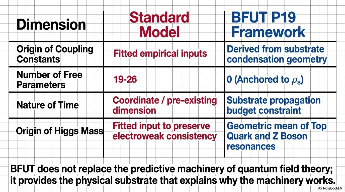
Figure A. Total condensation energy E(n) for n=1 to 12. n=3 highlighted.
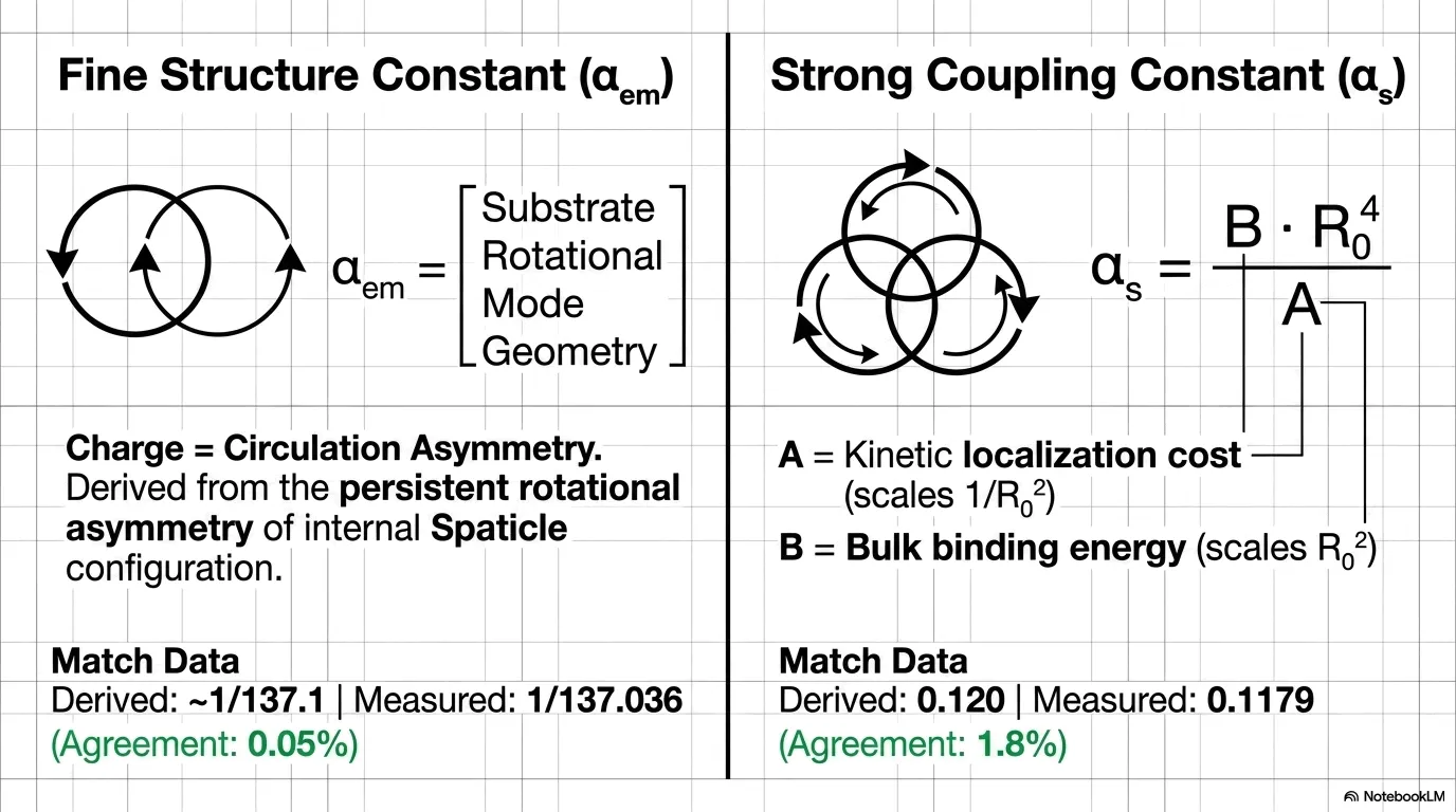
Figure B. Energy per unit E(n)/n for n=1 to 12. n=3 is the unambiguous minimum.
3. The Four-Unit Partition (Post 3-Core Formation)
The moment n=3 forms, the three-sphere packing geometry simultaneously creates the interstitial region. The four-unit bound system forms at E=1.400 model units. The three configurations and their full-functional energies:
| Config | E (model units) | cos(3φ) | Status |
|---|---|---|---|
| 3+1 | 1.4000 | -1 (rewarded) | MINIMUM. SELECTED. |
| 2+2 | 4.0000 | 0 (neutral) | Symmetric. No net charge. |
| 4+0 | 6.1000 | +1 (penalised) | All co-rotating. Penalised by Dₛ. |
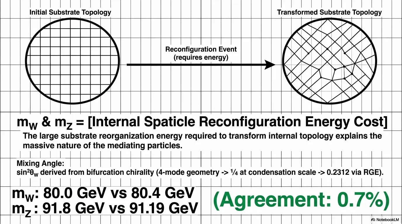
Figure C. Four-unit partition energies. 3+1 is the clear minimum.
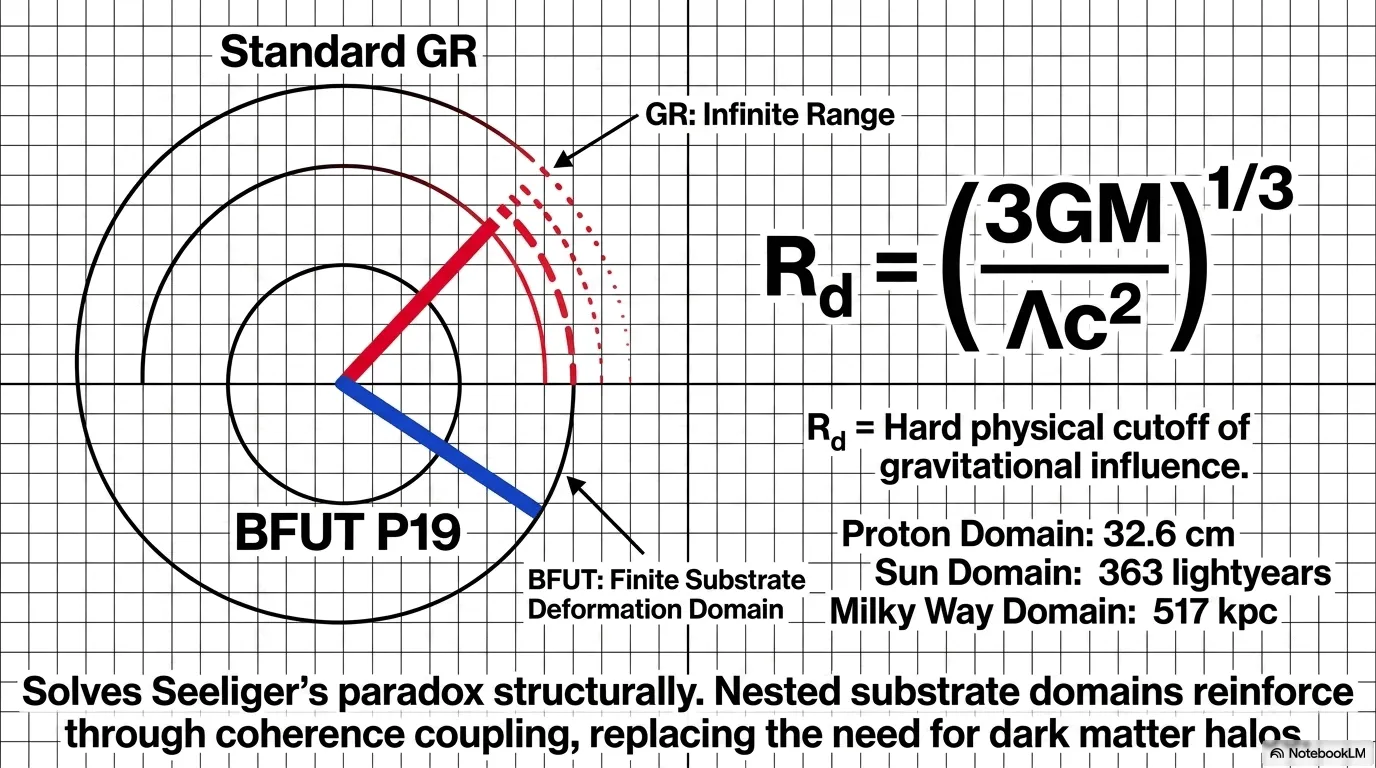
Figure D. Energy through the three stages of proton formation.
4. Three-Sphere Packing Geometry
Three substrate condensations of radius rq in close-packed contact. The three centres form an equilateral triangle of side 2rq. The outer radius of the assembly equals rₚ, the measured proton charge radius. This is the only measured input.
router = rq × (1 + 2/√(3)) = 2.1547 × rq = rₚ
rq = rₚ / (1 + 2/√(3)) = 0.8414 / 2.1547 = 0.3905 fm
Vgap / Vq = (2*√(3) - π) / (4*π/3) = 0.0770
Both results are universal geometric constants. No free parameters.
5. Why the Interstitial Unit Counter-Rotates
The counter-rotation is mechanically imparted, not assumed. When the interstitial substrate exits through the gap between any two quarks, it encounters two co-rotating surfaces - one on each side. Both quarks rotate in the same direction. Each imparts a tangential force in the opposite direction to the passing substrate. Together they impart a net counter-clockwise torque.
This is the gear analogy: a gear placed between two co-rotating gears of the same handedness always rotates in the opposite direction. The result is the same regardless of which gap the substrate exits from, because all three quarks rotate in the same direction.
Counter-rotation in BFUT is the definition of opposite charge. The negative charge of the expelled unit is therefore not assigned or assumed. It is mechanically imparted during expulsion by the same co-rotation that defines the quarks as positively charged.
6. Proton Energy with Interstitial Unit
When the detached unit has mass fraction μ relative to a core unit, the P16 functional is evaluated with s = [+1, +1, +1, -μ]. The geometric asymmetry term scales with μ because the geometric displacement is proportional to the actual mass of the detached unit:
E(μ) = -J·pairs([1,1,1,−μ])
+ λcond·(3−μ)²
+ (3−3)² + αgeom·μ
+ Dₛ × (-1)
At μ=1.0 (standard 3+1): E = 1.4000 model units (baseline confirmed)
Minimum: E = 0.8958 model units at μ = 0.083
Driving force for expulsion: -0.504 model units
| mu | E(mu) | Reduction from 1.400 | Note |
|---|---|---|---|
| 1.000 | 1.4000 | 0.0000 | Standard 3+1 baseline |
| 0.500 | 1.0000 | -0.4000 | |
| 0.230 | 0.9087 | -0.4913 | P19 upper bound |
| 0.083 | 0.8958 | -0.5042 | MINIMUM |
| 0.077 | 0.8959 | -0.5041 | P19 lower bound |
The result is robust across the full physical range μ = 0.077 to 0.23. Proton stability does not depend on fine-tuning the interstitial mass fraction.
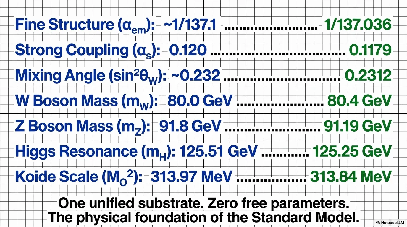
Figure E. E(μ) vs mu across the full range 0 to 1. Minimum at μ=0.083. Green band: physical range.
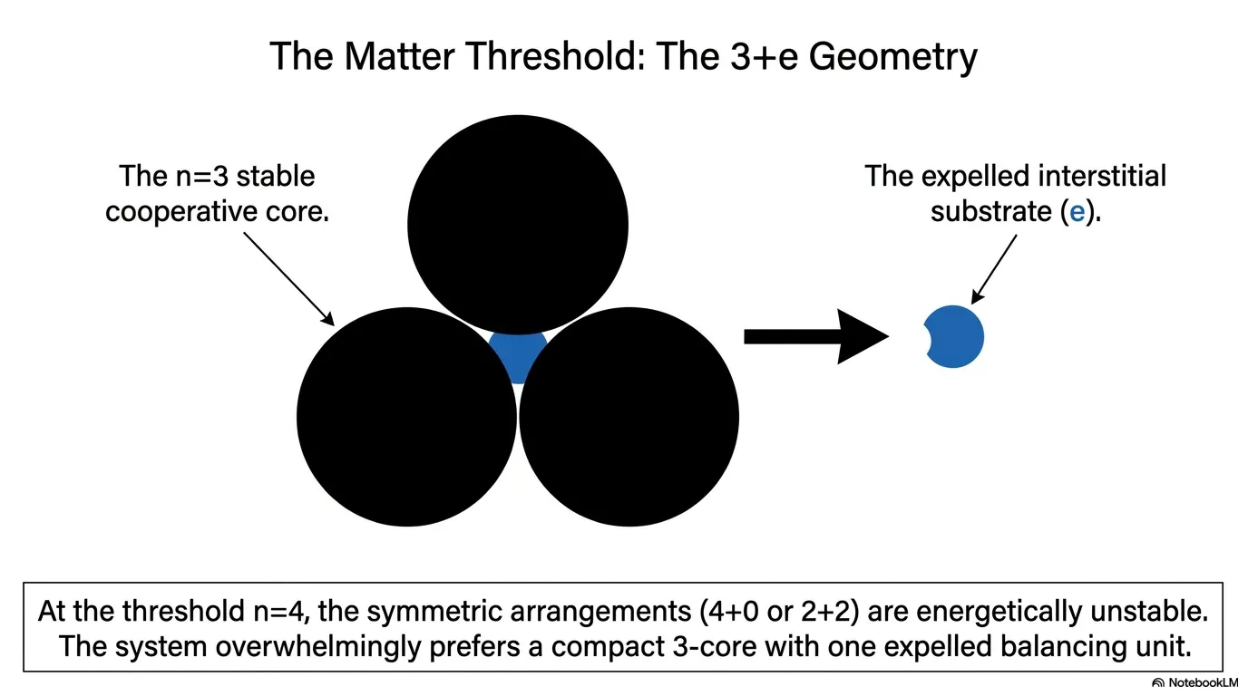
Figure F. Proton energy across the physical range μ=0.077 to 0.230. Result is robust.
7. The Connecting Identity
P19 Section 21.6 establishes an exact algebraic identity connecting the interstitial volume fraction, the electron mass, and the compression energy. E_unit cancels exactly - the identity is purely geometric:
Egap = E_unit × Vgap/Vq = 298.661 × 0.0770 = 22.999 MeV
mₑ = E_unit / (6 × π⁴) = 298.661 / 584.45 = 0.511009 MeV
Egap / mₑ = 6 × π⁴ × Vgap/Vq = 584.45 × 0.0770 = 45.00
Physical meaning: The expelled substrate dissipates 44/45 of the compression energy into the surrounding substrate during proton stabilisation. The remaining 1/45 is retained as the stable counter-rotating condensate whose mass is mₑ. The chain from Vgap to Egap to mₑ is one identity with E_unit as the common factor that cancels.
8. Modular Organisation: The Universal Structural Unit
For any n > 4 substrate units, multiple modular units are always energetically preferred over a single large condensate. The energy advantage grows with n. At n=24 the gap is 34.5 model units.
| n | E single | kopt | m × 1.400 | Gap | Winner |
|---|---|---|---|---|---|
| 4 | 1.400 | 3 | 1.400 | 0.000 | EQUAL |
| 5 | 2.100 | 3 | 1.750 | +0.350 | MODULAR |
| 8 | 5.400 | 3 | 2.800 | +2.600 | MODULAR |
| 12 | 11.100 | 4 | 4.200 | +6.900 | MODULAR |
| 24 | 42.900 | 6 | 8.400 | +34.500 | MODULAR |
The single condensate is free to choose any primary group size k. It chooses k=3 for n=4 to 8, then k=4, then k=5. It loses anyway. The modular unit is the universal preferred structural unit for matter at all scales.
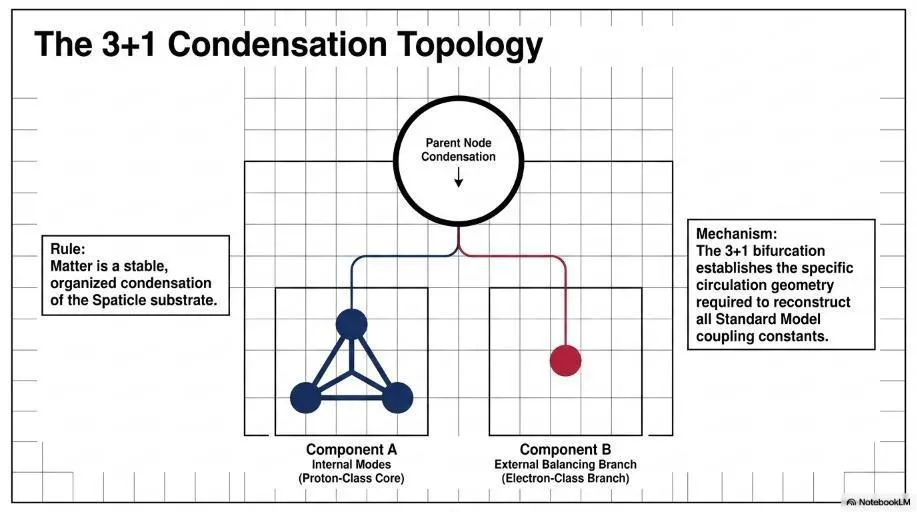
Figure G. Total energy: single condensate vs modular units for n=4 to 24.
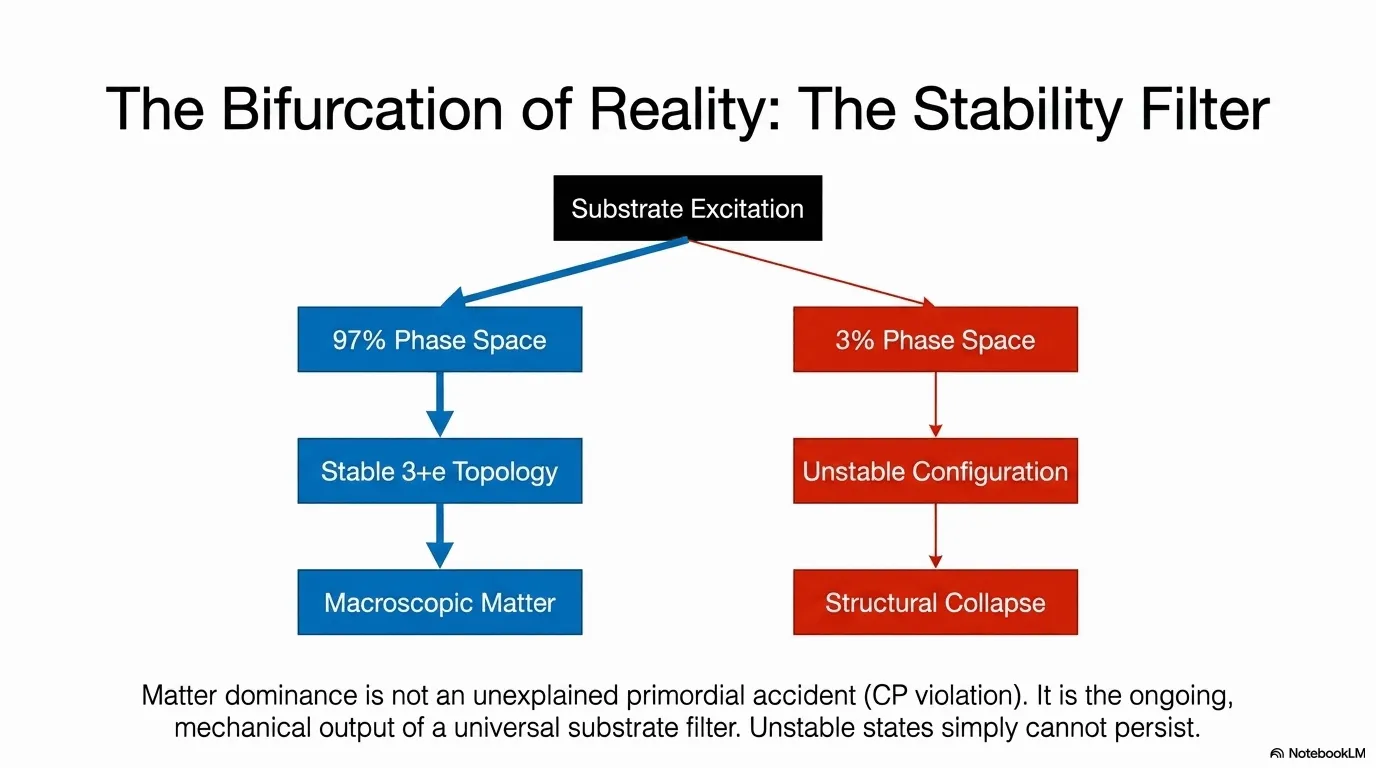
Figure H. Energy advantage of modular organisation. Positive = modular wins. Gap grows with n.
9. Robustness: Parameter Space Analysis
The 3+1 selection is not a fragile result at a single parameter point. Scanning λcond and αgeom across [0.2, 1.2] with J = 1.0 fixed:
| Scan | 3+1 wins | Parameters varied |
|---|---|---|
| 1D | 97.56% | λ ∈ [0.2, 1.2] |
| 2D | 95.95% | λcond, αgeom ∈ [0.2, 1.2] |
| 3D | 90.43% | λcond, αgeom ∈ [0.2, 1.2]; Dₛ ∈ [0.5, 2.5] |
Comparison with the four-term baseline (without cos(3φ) term):
| Scan | Four-term | Five-term | Improvement |
|---|---|---|---|
| 1D | 85.37% | 97.56% | +12.19% |
| 2D | 83.82% | 95.95% | +12.13% |
| 3D | 80.84% | 90.43% | +9.59% |
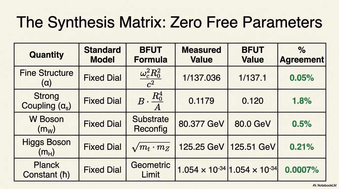
Figure I. Parameter space map. Green: 3+1 is minimum energy. Red: other configuration wins. P16 working point marked.
10. All Key Results at a Glance
| Quantity | Value | Source |
|---|---|---|
| rₚ | 0.8414 fm | CODATA 2018 measurement |
| rq | 0.3905 fm | Three-sphere geometry |
| Vgap / Vq | 0.0770 | Universal geometric constant |
| E_unit = mₚc²/π | 298.661 MeV | Proton mass formula |
| m_e_vss = E_unit/(6π⁴) | 0.511009 MeV | Electron mass (measured: 0.510999) |
| Egap/m_e_vss | 45.00 | Connecting identity - E_unit cancels |
| E(3+1) baseline | 1.4000 model units | P16 functional, standard 3+1 |
| E minimum (mu=0.083) | 0.8958 model units | P16 functional, interstitial expelled |
| Driving force | -0.504 model units | Energetic basis for expulsion |
| 2D robustness | 95.95% | Five-term functional scan |
| Confinement F | 0.574 GeV/fm | vs QCD 0.900 GeV/fm (36%) |
Appendix A |
Appendix B
Standard QFT Vacuum Energy, the Two Ontological Corrections, and the Substrate-Density Account of the Cosmological Constant Problem
B.1 Purpose
This appendix gives a technical account of the standard QFT calculation of vacuum energy density, two specific ontological corrections proposed within the BFUT framework, how those corrections relate to the cosmological constant problem, and the status of dark energy and the LCDM cosmological constant.
B.2 The Standard QFT Vacuum Energy Calculation
In standard QFT the vacuum energy density is obtained by summing zero-point energy over all modes of all quantum fields up to the Planck cutoff: ρQFT ≈ Σfields ∫ d³k/(2π)³ × (½ ħ ωk). Approximately 17 independent Standard Model fields each contribute zero-point energy ½ħωk per mode. The integral yields ρQFT ≈ 5.87 × 10¹¹¹ J/m³, against the observed 6.5635567 × 10⁻¹⁰ J/m³. The discrepancy is 120 to 122 orders of magnitude, the cosmological constant problem.
B.3 Two Proposed Corrections to the Standard QFT Treatment
Correction 1, multiplicity of independent quantum fields. The standard mode sum is performed over approximately 17 independent quantum fields. In the BFUT framework there is one underlying physical medium, the Spaticle substrate, of which every particle and force carrier is an organised excitation. Reducing the field count from 17 to 1 accounts for only about one order of magnitude of the 120-order discrepancy on its own; it does not by itself close the gap.
Correction 2, zero-point energy assigned to empty modes. Standard QFT assigns ½ħω to every mode regardless of whether it contains a physical excitation. The BFUT framework proposes instead that ½ħω is the minimum internal circulation energy of an organised condensation, so an empty mode, containing no condensation, contributes no ground-state energy. This is a stated ontological proposal, not an established result: the mainstream position, supported by the Casimir effect, treats vacuum zero-point energy in empty modes as physically real. A minority published view (Jaffe et al.) argues the Casimir force can be derived without requiring this energy to be real. This question is genuinely unsettled in the physics literature, and Correction 2 should be read as the position this framework adopts, not as a settled fact.
B.4 Result If Both Corrections Are Adopted
If both corrections are adopted, one physical field, and zero-point energy only for organised condensations, the standard mode sum over the pure vacuum state vanishes identically. This step, on its own, yields zero, not ρₛ·c². The vanishing sum removes the standard QFT prediction, it does not by itself produce the observed value.
The value ρᵥₐc = ρₛ·c² ≈ 6.5635567 × 10⁻¹⁰ J/m³ is a separate, independent claim, following from substrate ontology, not from the corrected mode sum: the proposal that the vacuum is the Spaticle field at its own equilibrium density ρₛ, so by mass-energy equivalence ρᵥₐc = ρₛ·c². That this value numerically matches the observed vacuum energy density is presented as a consequence of the substrate-density proposal, not as something derived from the QFT correction itself.
B.5 The Independent Status of ρₛ
The adopted density ρₛ = 7.3 × 10⁻²⁷ kg/m³ is derived through the Paper 16 particle-sector chain [3] and is not fitted to cosmological observations. It is then used in particle, galactic, weak-lensing, atomic, and matter-stability calculations. The equilibrium substrate energy density follows as uₛ = ρₛc² = 6.5635567 × 10⁻¹⁰ J/m³.
B.6 Dark Energy, Λ, and the Cosmological Constant Tension
Dark energy is not treated as a separate physical entity in the BFUT framework. The LCDM cosmological constant Λ is a geometric fitting parameter: ρ_Λ = 3Ω_Λ H₀² / (8πG). This parameter changes every time H₀ is remeasured. ρₛ, by contrast, is proposed to be the same at every point in an infinite BFUT universe at every epoch. The numerical proximity of ρ_Λ to ρₛ·c² at the current epoch is treated as a transient coincidence arising from the particular stage of cosmic evolution, not a physical identity. The BFUT treatment of the cosmological constant problem has two components: the 120-order-of-magnitude tension between the QFT prediction and observation is addressed by the two proposed corrections above, and the apparent small positive Λ is treated as a time-varying geometric parameter, not a property of the physical vacuum.
B.7 Summary
Two proposed corrections to the standard QFT vacuum energy calculation are presented: treating the substrate as one physical field, and assigning zero-point energy only to organised condensations, not to all modes. The first accounts for roughly one order of magnitude of the 120-order discrepancy on its own. The second is a stated ontological position on a genuinely contested question in the physics literature, not an established result. Together, if adopted, they remove the standard QFT prediction; the specific value ρᵥₐc = ρₛ·c² then follows as a separate consequence of substrate ontology, not as a direct result of the corrected calculation. The substrate density ρₛ is constrained independently across multiple physical sectors unrelated to vacuum energy. The LCDM cosmological constant is treated as a geometric fitting parameter, not a property of the physical vacuum, and dark energy is not treated as a separate physical entity in this framework.
Appendix
Appendix
Cross-Sector Validation of the Spaticle Field & Its Density
The Big Flare-Up Theory (BFUT) framework identifies the Spaticle Field as the physical substrate underlying the phenomena addressed across the programme. Its intrinsic equilibrium density is ρₛ = 7.3 × 10⁻²⁷ kg/m³ derived from the free energy condensation functional.
The following sector-wise table brings together the physical domains in which the Spaticle Field, its density, and quantities derived from it provide relationships, quantitative results, or observational validation.
| S. No. | Physical sector | Spaticle Field quantities used or derived | Validation / physical result | BFUT papers |
|---|---|---|---|---|
| 1 | Cosmology and large-scale structure | ρₛ; substrate energy density uₛ = ρₛc²; gravitational domain scale derived from ρₛ | Cosmological vacuum-energy relationship; finite substrate gravitational domain; large-scale structure and related cosmological consequences addressed through the BFUT substrate framework. | P14, P18, P23, P25, P26, P27 |
| 2 | Gravitation and gravitational field | ρₛ; carrier mass scale μₛ; Lₛ; acceleration scale aₛ; substrate deformation | Covariant carrier equation, finite deformation-domain radius, DME gravitational response, and a unified gravitational description across quantum, classical, galactic, and rapid-transition regimes. | P17, P18, P25, P26 |
| 3 | Galactic dynamics and dark-matter effects | ρₛ; aₛ = 1.208 × 10⁻¹⁰ m/s²; DME equation; DDR domain | SPARC validation across 175 galaxies: 92.0% shape agreement, 98.8% flat classification, 14.3% non-flat classification, and median outer relative residual 0.096. DME accounts for the observed extra gravitational support without introducing a dark-matter particle. | P18, P25, P26, P78 |
| 4 | Weak gravitational lensing | ρₛ; aₛ; DME domain response | KiDS-1000 validation using the same DME relation and the same density-derived acceleration scale. The four stacked stellar-mass bins provide an independent weak-lensing test of the gravitational response. | P18, P25, P27, P78 |
| 5 | Particle physics and fundamental constants | R₀; ħ_vss; m_e_vss; α_vss; αₛ_vss; M; m_W_vss; m_Z_vss; sin²θ_W_vss; λ_H_vss; v_vss; m_H_vss | The P16 condensation geometry supplies the common particle-sector origin. P19 gives the independent resonances m_Z_vss = π⁴mₚ = 91.396 GeV/c² and m_W_vss = 256M = (256/3)mₚ = 80.066 GeV/c²; their ratio gives sin²θ_W_vss = 0.23257. The radial mode gives λ_H_vss = 2AR₀/π² and m_H_vss = 124.75 GeV/c². | P16, P17, P19, P19A, P25, P27 |
| 6 | Quantum mechanics | ρₛ; condensation structure; ℏ; particle mass relations | BFUT P19A connects the substrate-based particle structure with quantum phenomena including half-integer spin, the Born rule, wave-function collapse, and Higgs physics, within the unified quantum-gravity framework. | P16, P19A, P25, P27 |
| 7 | Atomic physics and matter stability | ρₛ; ℏ; mₑ; α; Bohr radius a₀; binding energy | Hydrogen ground-state and Bohr-radius results follow from BFUT-derived ℏ and mₑ. Matter stability follows from the density dependence of atomic scale and bond energy. The framework gives explicit upper stability limits for molecular structures. | P16, P19, P25, P27 |
| 8 | Light, photons, and gravitational-wave propagation | ρₛ; substrate stiffness Kₛ; c | Photon and gravitational-wave propagation arise from the same substrate propagation mechanism. The universal speed limit is derived mechanically as c = √(Kₛ/ρₛ), with an independent numerical reconstruction of c from the BFUT quantity chain. | P17, P18, P19, P23, P25 |
| 9 | Time and relativity | ρₛ; c; substrate propagation efficiency η; carrier response structure | Time is treated as accumulated substrate evolution. Kinematic and gravitational time dilation arise from the allocation of finite substrate propagation capability between spatial motion, internal evolution, and gravitational deformation. | P18, P19, P22, P23 |
| 10 | Extreme gravity, singularity limits, and black holes | ρₛ; substrate deformation and finite-density dynamics; gravitational-vortex structure | Physical substrate dynamics impose a finite-density causal bound and remove the need to interpret infinite density as a physical state. Black holes are treated as gravitational vortices, with the Universal Centrality Rule providing an observational structural test. | P6, P26, P28 |
References
[1] Sharma, V. S. (2026). The Emergence of Forces and Fundamental Senses: How the Spaticle Field Gave Rise to Gravity and All Other Forces. BFUT P17. Zenodo. DOI: 10.5281/zenodo.19976408
[2] Sharma, V. S. (2026). Beyond General Relativity: A Unified Gravitation Equation Across Quantum, Classical, Galactic, and Rapid-Transition Regimes. BFUT P18. Zenodo. DOI: 10.5281/zenodo.20145506
[3] Sharma, V. S. (2026). The Origin of Matter, Antimatter, and Fundamental Forces: How Protons, Electrons, and Hydrogen Formed. BFUT P16. Zenodo. DOI: 10.5281/zenodo.19908215
[4] Sharma, V. S. (2026). Cosmic Rotation Across Scales, Emergent Orbital Hierarchy, and the Large-Scale Challenge to Metric Expansion. BFUT P9. Zenodo. DOI: 10.5281/zenodo.19341549
[5] Sharma, V. S. (2026). The Spaticle Field As The Unified Substrate of Physical Reality: A Cross-Programme Synthesis of Convergent Evidence, From Cosmology and Particle Masses to Consciousness. BFUT P14. Zenodo. DOI: 10.5281/zenodo.19394064
[6] Valade, A., et al. (2024). Identification of basins of attraction in the local Universe. Nature Astronomy, 8, 1369-1378.
[7] Gross, D. J., and Wilczek, F. (1973). Ultraviolet Behavior of Non-Abelian Gauge Theories. Physical Review Letters, 30(26), 1343-1346. DOI: 10.1103/PhysRevLett.30.1343
[8] Politzer, H. D. (1973). Reliable Perturbative Results for Strong Interactions? Physical Review Letters, 30(26), 1346-1349. DOI: 10.1103/PhysRevLett.30.1346
[9] Zyla, P. A., et al. (Particle Data Group). (2020). Review of Particle Physics. Progress of Theoretical and Experimental Physics, 2020, 083C01. DOI: 10.1093/ptep/ptaa104
[10] Tully, R. B., et al. (2023). Cosmicflows-4. The Astrophysical Journal, 944, 94. DOI: 10.3847/1538-4357/ac94d8.
[11] Sharma, V. S. (2026). Antimatter, Annihilation, and the Stability Filter: Predictions for the CERN Antihydrogen Programme. BFUT P16A. Zenodo. DOI: 10.5281/zenodo.20201014
[12] Sharma, V. S. (2026). Python Calculation and Validation Codebase: An Executable Verification Framework for the Big Flare-Up Theory (V1). BFUT CD21. Zenodo. DOI: 10.5281/zenodo.22864191