
The Origin of Matter, Antimatter, and Fundamental Forces:
How Protons, Electrons, and Hydrogen Formed
Vijay Shankar Sharma
Independent Researcher, Gurugram, National Capital Region, India
vss@vijayshankarsharma.com | ORCID: 0009-0001-9622-6121
DOI: 10.5281/zenodo.19908215
The author declares no conflict of interest and no funding was received for this research.
License: CC BY-NC-ND 4.0
Abstract
This paper establishes the complete pre-hydrogen sequence within the Big Flare-Up Theory [6], from the first stable matter condensation through to the formation of the first atom, and derives the physical nature of several quantities the Standard Model treats as given, not explained. A free-energy functional derived from the Spaticle field identifies n=3 as the first stable cooperative core, and the three-core is shown to generate its own electron through the 3+e mechanism, with n=4 partition energies confirming this asymmetric arrangement is decisively preferred over symmetric alternatives. A dynamic assembly simulation traces the continuous physical route from this 3+e condensation to ordinary hydrogen (protium), the first atom in the BFUT sequence: the three-core maps to a proton through an effective role assignment of (+2/3, +2/3, -1/3), the generated unit maps to an electron of charge -1, and their combination is ordinary hydrogen.
Charge is shown to be a mechanical property, not a primitive one: it is fixed by the counter-rotation direction imparted by the gear geometry of the three-sphere packing, with the familiar fractional charges emerging from this role map, not assumed in advance. Mass is fixed by the same packing geometry through the connecting identity mₚ/(6π⁵) = 0.511009 MeV, and particle identity itself is explained structurally, since two electrons anywhere in the universe are identical because each is an independent realisation of the same stability minimum recreated from the same substrate at the same ρₛ.
The same stability analysis yields a direct physical mechanism for matter-antimatter annihilation and a structural account of the matter-antimatter asymmetry, without requiring an asymmetric initial condition. Robustness scans across one, two, and three-dimensional parameter space show the 3+e configuration is the minimum-energy outcome in 97.56%, 95.95%, and 90.43% of cases respectively; the remaining few percent, where a stable 3+e condensation does not form, is shown to generate its own cancellation wave at the moment of formation, identified here as the antiparticle. This derived stability hierarchy is further shown to be consistent with the experimental history of particle physics, in which unstable exotic multiquark configurations decay while ordinary proton-electron matter remains the dominant stable baseline across every explored energy scale.
The condensation scale at the centre of this derivation is independently confirmed by a second, unrelated route: substituting six physical constants (α, e, ε₀, mₚ, c, rₚ), of which c and e are SI-defined and the others are measured, into standard electromagnetism extracts R₀ = 1.27348831 with no BFUT assumptions, agreeing with the geometrically derived R₀ = 1.27348221 to 0.00048%. These two routes, each unaware of the other, converge on the same condensation scale, mutually validating the condensation functional and every result built upon it. The resulting framework is presented as a constructive existence proof and structured-threshold model under BFUT assumptions, not as a replacement for QCD or the Standard Model.
Keywords: Spaticle field; quark; BFUT; Big Flare-Up Theory; proton formation; electron mass; hydrogen formation; threshold logic; three-sphere packing; connecting identity; antimatter; stability filter; matter-antimatter asymmetry; modular organisation; substrate condensation; origin of fundamental forces; 3+e configuration
1. Introduction
The BFUT Layer 1 programme argues that ordinary hydrogen is the first stable atomic milestone in the infinite BFUT universe. The missing conceptual bridge has always been the route between the Spaticle field and hydrogen. That gap is the exact target of the present paper. The goal is not to replace all Standard Model mathematics. The goal is to show that once the vacuum is reinterpreted as a real substrate, a coherent continuous emergence chain becomes possible and physically meaningful.
The chain pursued here is intentionally strict. First, the Spaticle field must support a first stable localised subatomic excitation. Second, if the opportunity field remains sufficiently uniform, that same first excitation should continue to appear first. Third, repeated appearance of the same first unit should not itself create novelty. Fourth, when the first stable completion threshold is crossed, the system should reorganise into the first atomic architecture. This preserves the same one-thing-at-a-time logic that BFUT uses at larger scales.
The importance of this paper is therefore structural. The paper provides the formal microphysical foundation for the emergence of matter from the Spaticle field substrate. The connection to fundamental forces is direct: the 3+e topology establishes the charge separation between the three-core and the generated electron that is the physical precondition for electromagnetic interaction. The three-sphere packing geometry establishes the confinement geometry that is the physical precondition for the strong force. The stability filter asymmetry between 3+e and its inverse topology is the physical precondition for weak-force asymmetry.
A central claim of this paper is that the experimentally observed stability hierarchy of particle physics is not incidental. Over decades of accelerator experimentation, laboratories have produced a vast range of temporary hadronic and exotic matter states, yet ordinary proton-electron matter remains the dominant stable endpoint. This paper argues that the observed hierarchy follows naturally from the 3+e threshold stability structure derived here, providing a single substrate-level emergence principle beneath multiple otherwise separate theoretical descriptions.
The Big Flare-Up Theory (BFUT) identifies the real physical fabric of space as the Spaticle field. The density calculation begins with the dimensionless condensation equilibrium, uses measured proton radius and mass anchors to obtain the BFUT particle quantities, and applies the particle-sector energy-density identification described in Section 2. The adopted equilibrium density is ρₛ = 7.3 × 10⁻²⁷ kg/m³.
1.1 Symbols and Notation Used in This Paper
The following symbols are used throughout this paper. Values are from the BFUT Master Symbol Guide unless derived explicitly below. The equilibrium Spaticle field density used throughout is the particle-sector result ρₛ = 7.3 × 10⁻²⁷ kg/m³.
Provenance convention: a BFUT-derived standard quantity carries the exact _vss suffix where provenance is relevant. BFUT-specific quantities retain their reserved symbols without a provenance suffix. Measured inputs use their standard symbols. The labels identify provenance and do not change the underlying physical quantity.
| Symbol | Definition | Value / Expression |
|---|---|---|
| Fundamental Spaticle Field Constants | ||
| ρₛ | Intrinsic equilibrium density of the Spaticle field | 7.3 × 10⁻²⁷ kg/m³ |
| P16: Condensation Functional Symbols | ||
| E(n) | Total condensation energy for n units | |
| Dₛ | Circulation phase reward coefficient | 1.5 |
| φ | Circulation phase angle in P16 condensation | |
| E_unit | Fundamental energy unit | mₚ·c²/π = 298.661 MeV |
| Vgap/Vq | Interstitial volume fraction | |
| Shared Physical Constants | ||
| G | Gravitational constant | 6.674 × 10⁻¹¹ m³ kg⁻¹ s⁻² |
| c | Speed of light | 2.998 × 10⁸ m/s |
| ℏ | Reduced Planck constant | 1.055 × 10⁻³⁴ J·s |
| mₚ | Proton mass | 938.272 MeV/c² |
| mₑ | Electron mass | 0.510999 MeV/c². BFUT: mₚ/(6π⁵) = 0.511009 MeV (0.002%) |
| rₚ | Proton charge radius | 0.8414 fm (CODATA 2018). BFUT: R₀·ℓmodel = rₚ by construction (0.000%) |
2. Particle-Sector Derivation of the Spaticle Field Density and Physical Vacuum Energy
2.1 Particle-Sector Derivation
A, B, C and D are dimensionless condensation-functional coefficients. They determine the dimensionless equilibrium radius R₀, not ρₛ directly. The following calculation connects that radius to the particle sector using measured proton anchors and the BFUT relations, then identifies the equilibrium substrate energy density with a particle-sector gravitational energy-density scale.
Step 1. Dimensionless condensation equilibrium
A = 0.5; B = 0.56308; C = −1/3; D = 1
E(R) = A/R² + BR² + CR + D/R
R₀ = 1.27348221
The positive stationary radius is a minimum: d²E/dR² = 6A/R⁴ + 2B + 2D/R³ > 0 for R > 0. The dimensionless energy scans and coefficient treatment are unchanged.
Step 2. Measured proton anchors and physical length
The measured proton charge radius fixes the length scale, while the measured proton mass supplies the mass scale:
rₚ = 0.8414 × 10⁻¹⁵ m (CODATA 2018); mₚ = 1.67262192369 × 10⁻²⁷ kg
ℓmodel = rₚ/R₀ = 6.60708091 × 10⁻¹⁶ m
Here ℓmodel is the physical length represented by one model-radius unit; it is not the proton charge radius itself. The calculation also uses c = 299792458 m/s, e = 1.602176634 × 10⁻¹⁹ C, the measured ε₀ = 8.8541878128 × 10⁻¹² F/m and G = 6.67430 × 10⁻¹¹ m³ kg⁻¹ s⁻² as supplied dimensional inputs.
Step 3. BFUT reduced Planck constant
ħ_vss = mₚ cℓmodel/π = mₚ c rₚ/(πR₀)
ħ_vss = 1.05457687 × 10⁻³⁴ J s
Step 4. BFUT electron mass and fine-structure constant
The electron mass follows from the BFUT mass-ratio relation, using the same proton-mass anchor:
m_e_vss = mₚ/(6π⁵) = 9.10955518 × 10⁻³¹ kg
α_vss = e²/(4πε₀ħ_vss c)
α_vss = 0.00729731763044; α_vss⁻¹ = 137.036655199
The α value here is calculated using ħ_vss and the supplied electromagnetic inputs e and ε₀. It is not an independent determination of those electromagnetic inputs. In the remaining equations mₑ and α denote these BFUT-calculated values, not substituted measured electron values. Each quantity carrying the suffix _vss is a BFUT-derived value; its derivation uses measured values of other quantities, and the suffix keeps each derived value distinct from the measured value of the same quantity.
Step 5. Characteristic particle mass and classical electron radius
mₑ/α = 1.24834297 × 10⁻²⁸ kg
rₑ = αħ_vss/(mₑ c) = 2.81788728 × 10⁻¹⁵ m
The scale rₑ is the classical electron radius constructed from these inputs, equivalently the reduced Compton wavelength of mₑ/α. It is the geometric radius obtained from the BFUT particle-sector construction.
Step 6. Particle-sector gravitational self-energy density
Using the BFUT positive gravitational energy-density prescription with the 8π normalisation:
ug = G(mₑ/α)²/(8πrₑ⁴)
ug = 6.56355667 × 10⁻¹⁰ J m⁻³
This prescription and the identification ρₛ c² = ug supply the physical closure connecting the particle scale to the substrate.
Step 7. Equilibrium Spaticle-field mass density
ρₛ = ug/c² = G(mₑ/α)²/(8πrₑ⁴c²)
ρₛ = 7.30294170 × 10⁻²⁷ kg m⁻³
Adopted working value: ρₛ = 7.3 × 10⁻²⁷ kg m⁻³.
Displayed extra digits make the numerical chain reproducible. The adopted density is carried forward in every equation in which ρₛ appears.
2.2 Cosmological-Constant Reference and Particle-Sector Density
The cosmological-constant expression ρ_Λ = 3Ω_ΛH₀²/(8πG) gives approximately 5.9 × 10⁻²⁷ kg/m³ for the reference cosmological inputs. This expression contains the Hubble constant H₀, and multiple accepted values of H₀ are currently in use. The particle-sector derivation gives ρₛ = 7.3 × 10⁻²⁷ kg/m³, adopted as ρₛ = 7.3 × 10⁻²⁷ kg/m³ for all subsequent calculations.
The particle-sector density established above is the working value used throughout the remainder of this paper.
2.3 Physical Substrate Energy and the QFT Vacuum Sum
The physical equilibrium rest-energy density of the one Spaticle field is obtained separately by mass-energy equivalence:
uₛ = ρₛ c² = 6.56 × 10⁻¹⁰ J/m³
Standard vacuum-energy estimates sum a zero-point contribution over empty modes of many independent fields. The BFUT ontology makes two changes: there is one underlying physical field, and zero-point energy belongs to organised condensations. Under those assumptions the corrected pure-vacuum mode sum is:
ρQFT,corrected = 0
The corrected pure-vacuum mode sum is zero, while the one physical Spaticle field has a finite equilibrium rest-energy density. The one-field cosmological-constant scale survives this treatment. Using the particle-sector value ρₛ = 7.3 × 10⁻²⁷ kg/m³ gives uₛ = 6.56 × 10⁻¹⁰ J/m³, approximately 23.8% above the representative one-field cosmological scale of 5.30 × 10⁻¹⁰ J/m³. This is an order-of-magnitude proximity compared with the conventional QFT vacuum-energy discrepancy of more than 120 orders of magnitude [1].
3. Vijay's Law and the Six-Layer BFUT Context [10]
This paper is explicitly guided by the same cross-layer principle that binds the six-layer BFUT reality framework, of which BFUT is Layer 1. For the present derivation, the directly relevant operative form of Vijay's law is: whenever conditions are stable or predictably unstable at any scale in the universe, more evolved matter will manifest. [10]
This is already the logic claimed in BFUT at larger scales from the Spaticle field to ordinary hydrogen. There is no reason to assume that the same law should fail in the intermediate subatomic bridge. If the substrate is uniform enough to keep emitting the same first stable excitation, then repetition should persist until a new threshold is reached. When the threshold is reached, a more evolved structure should manifest. That is exactly the principle implemented here.
This makes the paper philosophically economical. It does not introduce a new special rule just for subatomic physics. It extends the same law downward and tests whether the logic remains intact. The result is that the logic does remain intact at the constructive-model level.
A persistent objection to any framework proposing a physically real substrate for space is that the Michelson-Morley experiment of 1887 is said to have ruled out all medium-based accounts of light propagation. This objection is not decisive, for two independent reasons. The second reason is specific to BFUT and has not previously been stated in the literature.
First: the experiment tests for drift, not for existence. The Michelson-Morley apparatus was designed to detect a difference in light travel time along two perpendicular arms arising from Earth's motion through a stationary mechanical ether. The nineteenth-century luminiferous ether was a preferred-frame background at absolute rest. The expected fringe shift was not found. What was excluded is precisely this: a medium that maintains a preferred rest frame detectable by electromagnetic measurements. The Spaticle field does not maintain such a frame. It is a Lorentz-compatible substrate whose local propagation laws, clocks, and rulers are co-determined by the same local substrate state. No embedded observer can detect drift through it. The Michelson-Morley null result is exactly what BFUT predicts.
Second: the experiment is constitutionally incapable of detecting Spaticle substrate motion even in principle. In the classical luminiferous ether picture, light is a wave in the ether and matter is a separate substance moving through it. This ontological separation is what makes ether drift detectable in principle. In BFUT this separation does not exist. Light is not a separate entity moving through the Spaticle field. Light is a propagating excitation of the Spaticle field. The quantity c is not the speed of light through the substrate - it is the maximum reorganisation and propagation rate of the substrate itself. Matter is also an excitation of the Spaticle field - organised condensations of the same substrate, as established throughout this paper. The mirrors in Michelson's apparatus, the beam-splitter, the light beams, and the observer are all excitations of the same Spaticle field. If the substrate were drifting, everything would drift together. There is no external reference against which the drift could be measured - no more than a person on a ship can detect the ship's uniform motion by measuring distances between objects fixed to the same ship. This account of light as substrate excitation and c as substrate propagation rate follows from the BFUT substrate construction.
The Michelson-Morley experiment therefore confirms the BFUT picture directly. A null result is the only possible result in a universe where light and matter are both excitations of the same physical medium. The result has been understood since 1905 as evidence that there is no ether. The correct understanding is that it is evidence that if a physical substrate exists, it must be one in which light and matter are excitations of the same medium. A substrate of the classical type - where light and matter are separate - is excluded. A substrate of the BFUT type - where both are excitations of the same field - is not excluded. It is the only type the null result is consistent with.
4. Spaticle-Field Nucleation of the First Quark
The first integrated layer reinterprets vacuum excitation as excitation of a real Spaticle-field substrate. A free-energy functional is constructed for the first stable localised finite-size excitation:
E(R) = A/R² + B·R² + C·R + D/R
The four terms are assigned clear roles. A/R² acts as a localisation or kinetic-like cost. B·R² acts as bulk displacement cost in the Spaticle ocean. C·R acts as a boundary or gradient cost. D/R acts as an internal circulation or confined-mode support term. The point of the functional is not to claim a final Lagrangian. The point is to ask whether a real substrate can naturally prefer a finite localised lump over both collapse and indefinite spread. This continuous nucleation functional determines the condensation radius R* and the SI length scale ℓmodel; the full five-term discrete functional deposited in the companion code archive (DOI: 10.5281/zenodo.20517866) operates on discrete unit counts and determines which partition topology is energetically preferred at the n = 4 threshold. The two functionals serve complementary physical roles and are both required for the complete P16 derivation chain.
Summary of Derived Quantities
| Quantity | BFUT result | Status |
|---|---|---|
| A | 1/2 | Geometric / normalisation result |
| B | 0.56308 | Derived filling-deficit ratio |
| C | −1/3 | Three-sector surface-expulsion term |
| D | 1 | Topological circulation term |
| R₀ | 1.27348 | Derived functional minimum |
| R₀ physical | 1.27349 | Physical comparison value |
| md/mu | 1.01267 | Derived void-filling area ratio |
| qd | −1/3 | Derived charge partition |
| qu | +2/3 | Derived charge partition |
| mₑ/mₚ | 1/(6π⁵) | Derived BFUT mass ratio |
| Tcrit | 29.69 K | Derived nucleation threshold |
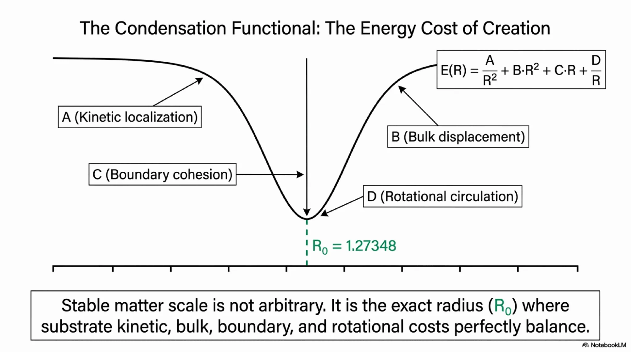
Figure 1. The condensation functional E(R) = A/R² + B·R² + C·R + D/R, showing the physical role of each term: A (kinetic localisation), B (bulk displacement), C (boundary cohesion), and D (rotational circulation), with stable minimum at R₀ = 1.27348.
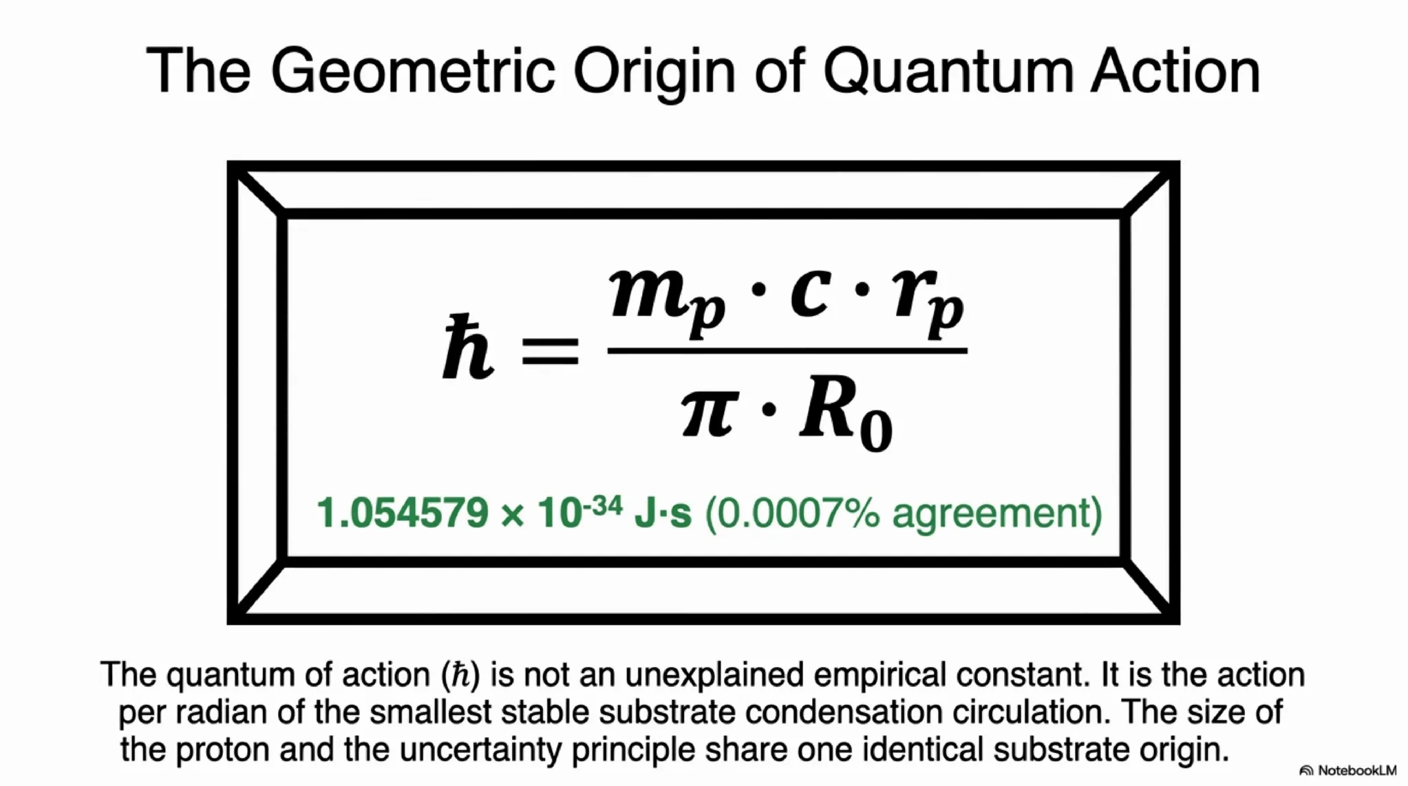
Figure 2. Robustness scan showing persistence of an interior non-zero nucleation minimum across 2D parameter space.
5. Physical Identification of the Coefficients and the SI Anchor
The four coefficients carry specific physical identities that connect the functional to the Spaticle field substrate. These identifications provide the physical mapping of the functional coefficients to substrate quantities: A = ħ² / (2 m_eff), the localisation or quantum kinetic cost, where m_eff is the effective mass of the condensation; B = (1/2) ρₛ cs² R₀², the bulk deformation cost, where ρₛ is the intrinsic equilibrium density of the Spaticle substrate and cs is the substrate propagation speed, equal to c by Lorentz compatibility; C = 4π R₀² σs in SI sketch form, with σs a signed boundary density. Void expulsion makes σs negative, so that C < 0. D = ωc × Icond, the internal circulation support, where ωc is the internal circulation frequency and Icond = (2/5) m_eff R₀² is the rotational inertia of the three-core.
R₀ = 1.27348. The quantum of action ħ is derived from the condensation geometry in Section 5.2.
The conversion from model units to SI uses one independently measured physical constant as an anchor: ℓmodel = rₚ / R₀ = 0.8414 fm / 1.27348 = 6.607 × 10⁻¹⁶ m, where rₚ = 0.8414 fm (CODATA 2018) is the proton charge radius. R₀ = 1.27348 is the minimum of E(R) with all four coefficients derived from first principles (see Appendix C), and agrees with the reconstruction rₚ·mₚ·c/(π·ħ) = 1.27349.
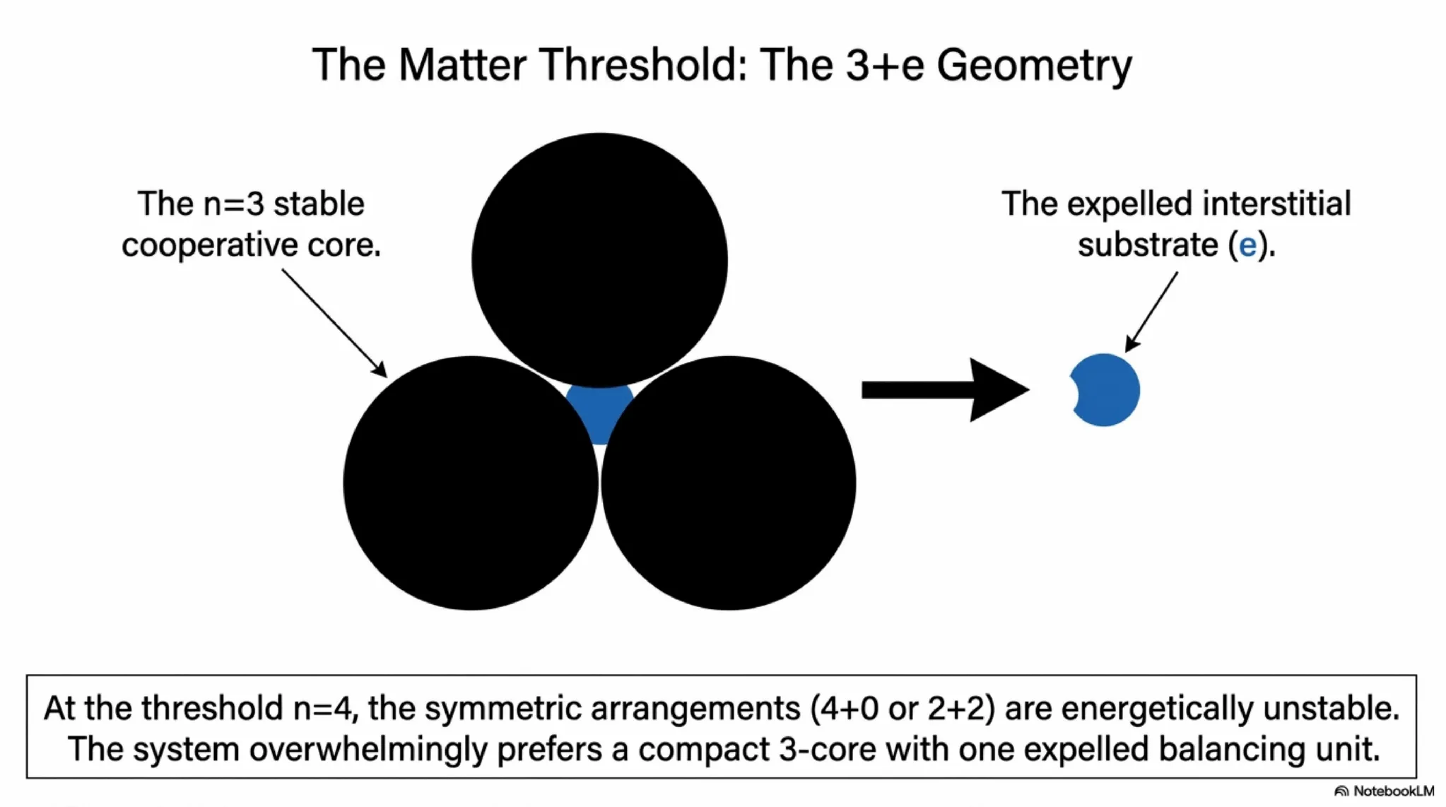
Figure 3. Geometric origin of the quantum of action: ħ = mₚ·c·rₚ/(π·R₀), matching the measured value to 0.00048%.
5.1 Density Dependence of Quantities Used in This Paper
The proton mass, electron mass, mass ratio, Bohr radius, hydrogen binding energy, and the A, B, C, D energy scan follow from the measured inputs and derived dimensionless condensation geometry displayed in this paper. Their final equations contain no ρₛ.
The quantities in P16 that contain ρₛ explicitly are the vacuum-stabilisation coefficient λSI = ρₛ/4, the equilibrium substrate rest-energy density ρₛ c², and the thermal-disruption normalisation and critical temperature. Their displayed equations use ρₛ = 7.3 × 10⁻²⁷ kg/m³.
This dependence test is algebraic: a quantity changes only when ρₛ survives in its final displayed equation. A narrative statement that a result comes from the substrate is not by itself a numerical dependence on ρₛ.
5.2 The Quantum of Action from Substrate Condensation Geometry
In 1900, Planck introduced what became Planck’s constant as an empirical constant required to fit blackbody radiation data. He proposed that oscillators exchange energy only in discrete amounts E = nhν, where n is an integer and ν is frequency, and determined the value of h by fitting the observed spectrum. The reduced form ħ = h/2π appeared subsequently in angular-frequency formulations through E = ħω. Planck did not derive ħ from deeper physics. Quantum mechanics subsequently adopted it as a fundamental postulate. Its numerical value has never been explained from more primitive physics within the standard framework.
In BFUT, ħ is not a primitive constant but a quantity whose numerical value emerges from substrate condensation geometry. This is structurally identical to the BFUT treatment of the fine structure constant α. Historically α ≈ 1/137 was measured. Likewise, Planck measured ħ_vss derives its numerical value from condensation geometry, as shown below. In both cases BFUT is not re-measuring a constant. It is explaining why that constant has the numerical value it does.
The SI anchor of Section 5 establishes the characteristic condensation length scale: ℓmodel = rₚ / R₀ = 0.8414 fm / 1.27348 = 6.607 × 10⁻¹⁶ m, where R₀ = 1.27348 is the derived condensation radius (functional minimum; verification: rₚ·mₚ·c/(π·ħ) = 1.27349), and rₚ = 0.8414 fm (CODATA 2018) is the independently measured proton charge radius. The proton mass mₚ = 938.272 MeV/c² is the characteristic condensation mass scale established through E_unit = mₚ c²/π in Appendix C, Section 9.1. The product mₚ·c is the characteristic momentum of the first stable substrate condensation. Multiplying by ℓmodel gives a quantity with the dimension of action:
(mₚ·c) × ℓmodel [kg·m/s·m = kg·m²/s = J·s]
which is precisely the dimension of ħ. Dividing by π, which enters through the proton mass threshold relation E_unit = mₚ c²/π established in Appendix C, Section 9.1:
Once R₀ is fixed by the condensation minimum and rₚ and mₚ provide the physical proton scale, the BFUT relation determines the corresponding ħ scale:
ħ_vss = mₚ·c·ℓmodel / π = mₚ·c·rₚ / (π·R₀)
Substituting the known values mₚ = 938.272 MeV/c², rₚ = 0.8414 fm (CODATA 2018), R₀ = 1.27348:
ħ_vss = 1.054577 × 10⁻³⁴ J·s
Measured value: ħ = 1.054572 × 10⁻³⁴ J·s. Relative difference: 0.00048%. R₀ = 1.27348 is the minimum of E(R) with all four coefficients derived from first principles (see Appendix C), and agrees with the reconstruction rₚ·mₚ·c/(π·ħ) = 1.27349.
Independent Empirical Validation of R₀ and the Condensation Functional
R₀ = 1.27348 is derived above from the condensation functional E(R) = A/R² + B·R² + C·R + D/R by setting dE/dR = 0, with all four coefficients A, B, C, D derived from first principles. No measured physical constants enter this derivation. The condensation scale falls out of pure substrate geometry.
An entirely independent empirical route to R₀ exists using independently measured physical constants and no BFUT-derived value of ħ. Using the standard relation α_meas = e²/(4πε₀ħ_meas c), the measured reduced Planck constant gives the direct reconstruction R₀ = mₚ·c·rₚ/(π·ħ_meas):
independently reconstructed R₀ = mₚ·c·rₚ/(π·ħ)
Substituting the independently measured values ħ = 1.054572 × 10⁻³⁴ J·s, mₚ = 1.6726 × 10⁻²⁷ kg, c = 2.998 × 10⁸ m/s, and rₚ = 0.8414 fm (CODATA 2018):
independently reconstructed R₀ = 1.27348831
This independently reconstructed value agrees with the geometrically derived R₀ = 1.27348221 to 0.00048%.
The significance of this agreement cannot be overstated. The first route uses no measured constants - it derives R₀ from the geometry of the condensation energy landscape alone. The second route uses no BFUT geometry - it extracts R₀ from standard electromagnetism and six physical constants (c and e SI-defined; α, ε₀, mₚ, rₚ measured). These two routes know nothing of each other. They arrive at the same condensation scale to within experimental precision.
The agreement provides an independent empirical check of the condensation scale. Quantities subsequently derived within BFUT should retain their BFUT provenance labels, while measured quantities used for comparison should retain measured provenance labels.
The physical reading of the formula is direct. The quantum of action is the characteristic momentum of the first stable substrate condensation, mₚ·c, multiplied by the characteristic condensation length scale, ℓmodel, divided by π. In words: ħ is the action associated with one condensation-scale momentum quantum traversing one condensation-scale length. The quantum of action has its numerical value because matter condenses at the scale set by the P16 free-energy functional.
The coefficient A = ħ²/(2m_eff) in the condensation functional is not a circular insertion of quantum mechanics into the substrate picture. In the displayed chain, ħ follows from the condensation geometry above, while m_eff = ħ/(c·ℓmodel) = mₚ/π follows algebraically from the measured proton scale and ℓmodel.
5.2.1 Action Quantisation: What ħ Physically Is
The BFUT ħ derivation identifies the quantum of action with a specific physical process. The action of one complete circulation of a substrate condensation at the condensation scale is:
S = m_eff·c·2π·ℓmodel = 2πħ = h
where m_eff = ħ/(c·ℓmodel) is the effective carrier mass established in the condensation construction, and h = 2πħ = 6.626 × 10⁻³⁴ J·s is Planck’s constant. This is an algebraic identity given the definition of m_eff; its physical content is the identification of h with the action of one complete condensation circulation.
Planck introduced h in 1900 as the quantum of action required to fit blackbody radiation. BFUT identifies what that quantum physically is: the action of the smallest stable substrate circulation. The factor 2π is the geometric factor for one complete cycle. ħ = h/2π is therefore the action per radian of circulation.
The minimum stable circulation quantum is Lmin = (1/2)·m_eff·c·ℓmodel = ħ/2. The factor 1/2 follows from the 720° restoration property of the 3+e condensation: the condensation requires two full frame rotations to return to its original configuration. The quantum of action ħ is therefore twice the minimum circulation quantum:
ħ = 2·Lmin [action quantum = twice minimum condensation circulation]
The factor of 1/2 that appears in Amodel = 1/2 (Section 5.4), in spin-1/2, and in Lmin = ħ/2 arises from the same 720° embedding topology of the first stable condensation.
5.2.2 The Fine Structure Constant from the ħ Derivation
Once ħ is derived in Section 5.2, the fine structure constant follows by substituting the BFUT expression for ħ into the standard electromagnetic definition. No additional step or new physical input is required.
The standard definition is:
α = e² / (4πε₀ħc)
Substituting ħ_vss = mₚ·c·rₚ/(π·R₀):
α = e² / (4πε₀·[mₚ·c·rₚ/(π·R₀)]·c)
= e²·π·R₀ / (4π·ε₀·mₚ·c²·rₚ)
= e²·R₀ / (4ε₀·mₚ·c²·rₚ)
Substituting the known values e = 1.602176634 × 10⁻¹⁹ C (exact), ε₀ = 8.8542 × 10⁻¹² F/m, mₚ = 1.67262 × 10⁻²⁷ kg, c = 2.99792 × 10⁸ m/s, rₚ = 0.8414 × 10⁻¹⁵ m, R₀ = 1.27348:
α_vss = 0.0072973 = 1/137.037
Measured: α = 1/137.036 | Difference: 0.00048%
The inputs are e and c (exact by SI definition), ε₀ and mₚ (measured), and rₚ = 0.8414 fm (CODATA 2018). Under the 2019 SI, ε₀ = e²/(2αhc), so this relation is the electromagnetic form of the condensation identity of Section 5.2: α_vss and ħ_vss reproduce α and ħ at the same 0.00048%.
The ħ residual, the two-route R₀ comparison, and the fine-structure comparison are the same 0.00048%, because ħ_vss, R₀, and α_vss are linked by one exact relation.
5.2.3 Planck-Charge Interpretation of the Fine-Structure Constant
The derivation of the fine-structure constant in Section 5.2.2 admits an additional physical interpretation through the Planck charge. This does not constitute a separate derivation of α_vss. Rather, it exposes the electromagnetic charge scale already contained in the BFUT-derived ħ_vss relation.
The conventional Planck charge in SI units is
qₚ = √(4πε₀ħc).
Since BFUT derives the reduced Planck constant from the condensation geometry,
ħ_vss = mₚcrₚ/(πR₀),
the corresponding Planck-charge value constructed using the BFUT-derived action scale is
qₚ_vss = √(4πε₀ħ_vss c).
Substitution of the BFUT expression for ħ_vss gives
qₚ_vss = √[4πε₀c · mₚcrₚ/(πR₀)]
and therefore
qₚ_vss = √(4ε₀mₚc²rₚ/R₀).
The fine-structure relation derived in Section 5.2.2 is
α_vss = e²/(4πε₀ħ_vss c).
Because
qₚ_vss² = 4πε₀ħ_vss c,
the same relation can be written directly as
α_vss = e²/qₚ_vss² = (e/qₚ_vss)².
Equivalently,
α_vss⁻¹ = (qₚ_vss/e)².
This provides a useful physical interpretation of the inverse fine-structure constant. Within the BFUT derivation chain, α_vss⁻¹ expresses the squared ratio between the Planck-charge scale constructed from ħ_vss and the elementary charge e.
Using the Section 5.2.2 value α_vss⁻¹ = 137.036655,
qₚ_vss/e = 1/√α_vss = √(α_vss⁻¹) ≈ 11.7063,
whose square gives
(qₚ_vss/e)² = α_vss⁻¹ = 137.036655.
The Planck-charge formulation therefore makes explicit a relationship already contained in the Section 5.2.2 derivation:
condensation geometry → R₀ → ħ_vss → qₚ_vss → α_vss.
The significance of this reformulation is that the BFUT-derived quantum action scale determines a corresponding electromagnetic charge scale once ε₀ and c are supplied. The same α_vss previously written as
α_vss = e²R₀/(4ε₀mₚc²rₚ)
is equivalently expressed as the squared charge ratio
α_vss = (e/qₚ_vss)².
No additional physical input is introduced by this representation. The quantities e and ε₀ retain the same status as the electromagnetic inputs used in Section 5.2.2. In particular, qₚ_vss is not an independently supplied scale; it is constructed from the already-derived ħ_vss together with ε₀ and c.
The Planck-charge relation is therefore not an independent determination of α_vss, but an equivalent representation of the same derivation. It clarifies the physical meaning of the resulting dimensionless coupling within this framework: α_vss measures the squared ratio of the elementary electric charge to the electromagnetic charge scale associated with the BFUT-derived quantum of action.
5.2.4 High-Precision Recalculation Using CODATA 2022
The particle-sector calculation used throughout this paper is based on the CODATA 2018 proton inputs together with the working numerical values B = 0.56308 and R₀ = 1.27348221. These give ħ_vss = 1.05457687 × 10⁻³⁴ J·s and α_vss⁻¹ = 137.036655199. This subsection does not replace those working values. It provides a separate higher-precision evaluation of the BFUT geometry and tests the resulting fixed geometry against the later CODATA 2022 constants.
High-Precision Evaluation of B and R₀
The coefficient B can be evaluated directly from the filling-deficit geometry given in the Appendix rather than being truncated to B = 0.56308. The geometric expression gives
B = 0.5630820806583208122552771497…
For A = 1/2, C = −1/3 and D = 1, the radial condensation functional is
E(R) = A/R² + BR² + CR + D/R.
Its stationarity condition is
dE/dR = −1/R³ + 2BR − 1/3 − 1/R² = 0,
or equivalently,
2BR⁴ − R³/3 − R − 1 = 0.
Using the high-precision value of B gives the positive stationary root
R₀ = 1.2734805699911956289979049003…
This value is determined entirely by the BFUT condensation geometry. It is held fixed throughout the following calculations and is not reconstructed or refitted from the CODATA 2022 physical constants.
Recalculation with CODATA 2022 Central Values
The calculation is performed in exactly the same direction as the original CODATA 2018 particle-sector calculation. The measured proton charge radius establishes the physical length scale,
ℓmodel = rₚ/R₀,
after which the BFUT reduced Planck constant follows as
ħ_vss = mₚcℓmodel/π = mₚcrₚ/(πR₀).
For the CODATA 2022 comparison the inputs are
mₚ = 1.67262192595(52) × 10⁻²⁷ kg,
rₚ = 0.84075(64) fm,
and
ε₀ = 8.8541878188(14) × 10⁻¹² F/m.
The ε₀ value in this calculation is therefore the CODATA 2022 value, not the CODATA 2018 value used in the working calculation elsewhere in this paper.
Using the fixed high-precision BFUT value of R₀ gives
ħ_vss(2022) = 1.053763541491691 × 10⁻³⁴ J·s.
The CODATA 2022 comparison value is
ħ = 1.054571817… × 10⁻³⁴ J·s,
giving
Δħ/ħ = (ħ_vss − ħ)/ħ = −0.07664496% = −766.450 ppm.
The BFUT fine-structure constant is then calculated from the same relation used in the original particle-sector calculation:
α_vss = e²/(4πε₀ħ_vss c).
This gives
α_vss(2022) = 0.00730294990741449
and
α_vss⁻¹(2022) = 136.93096798935.
The corresponding CODATA 2022 values are
α = 0.0072973525643(11)
and
α⁻¹ = 137.035999177(21).
Therefore,
Δα/α = (α_vss − α)/α = +0.07670375% = +767.038 ppm.
Thus, when the high-precision BFUT geometry is held fixed and the CODATA 2022 proton central values are substituted into the same calculation used previously with the CODATA 2018 inputs, the resulting central-value discrepancy is larger than in the 2018 comparison.
For a direct like-for-like comparison, the CODATA 2018 inputs can also be recalculated using the same high-precision R₀. This gives
ħ_vss(2018, high precision) = 1.05457822493 × 10⁻³⁴ J·s
and
Δħ/ħ = +0.00060757% = +6.076 ppm.
This high-precision 2018 comparison value should not be confused with the working value used elsewhere in the paper, ħ_vss = 1.05457687 × 10⁻³⁴ J·s, which was obtained using the original truncated B = 0.56308 and R₀ = 1.27348221. The working calculations in the body of the paper are not changed by this subsection.
| Calculation | R₀ treatment | Δħ/ħ |
|---|---|---|
| 2018 working calculation used in the paper | R₀ = 1.27348221 | ≈ +0.00048% |
| 2018 inputs with high-precision geometry | R₀ = 1.2734805699911956… | +0.00060757% |
| 2022 central inputs with high-precision geometry | Same fixed R₀ | −0.07664496% |
The direction of the displacement also changes. With the 2018 proton inputs, ħ_vss lies slightly above the measured value of ħ. With the CODATA 2022 central proton inputs, ħ_vss lies below it. Since B and R₀ are held unchanged between the two high-precision calculations, the change arises from the experimental input set, predominantly from the lower CODATA 2022 proton charge-radius central value.
Sensitivity Within the CODATA 2022 Uncertainty Range
The calculation using the CODATA 2022 central values is the primary 2022 comparison. A separate sensitivity calculation can determine the closest result obtainable within the individually quoted 1σ uncertainty intervals of the proton charge radius and proton mass.
Since ħ_vss ∝ mₚrₚ and the central 2022 result lies below ħ, the favorable direction within these intervals is toward the upper 1σ values:
rₚ(+1σ) = 0.84139 fm
and
mₚ(+1σ) = 1.67262192647 × 10⁻²⁷ kg.
Using these values while leaving the BFUT geometry unchanged gives
ħ_vss(+1σ) = 1.054565693073252 × 10⁻³⁴ J·s
and
Δħ/ħ = −0.00058076% = −5.808 ppm.
The corresponding fine-structure calculation gives
α_vss(+1σ) = 0.00729739494497188,
α_vss⁻¹(+1σ) = 137.03520332129,
and
Δα/α = +0.00058077% = +5.808 ppm.
This +1σ calculation is a sensitivity bound, not an alternative CODATA 2022 result. The primary 2022 comparison remains the calculation using the CODATA 2022 recommended central values.
| Quantity | 2018 inputs, high-precision R₀ | 2022 central values | 2022 favorable +1σ sensitivity bound | CODATA 2022 |
|---|---|---|---|---|
| ħ_vss (J·s) | 1.05457822493 × 10⁻³⁴ | 1.05376354149 × 10⁻³⁴ | 1.05456569307 × 10⁻³⁴ | 1.054571817… × 10⁻³⁴ |
| Δħ/ħ | +0.00060757% | −0.07664496% | −0.00058076% | 0 |
| α_vss | 0.00729730823 | 0.00730294991 | 0.00729739494 | 0.0072973525643(11) |
| Δα/α | ≈ −0.0006076% | +0.07670375% | +0.00058077% | 0 |
| α_vss⁻¹ | 137.03683168 | 136.93096799 | 137.03520332 | 137.035999177(21) |
The uncertainty in this test is overwhelmingly controlled by the proton charge radius. The relative standard uncertainty of the CODATA 2022 proton mass is approximately 3.1 × 10⁻¹⁰, whereas that of the proton charge radius is approximately 7.6 × 10⁻⁴. Consequently, movement of mₚ across its quoted uncertainty interval has a negligible effect on ħ_vss compared with movement of rₚ.
The radius corresponding to exact equality can be obtained directly by inverting the BFUT relation:
rₚ(BFUT) = πR₀ħ/(mₚc).
Using the CODATA 2022 proton-mass scale gives
rₚ(BFUT) ≈ 0.841395 fm.
Relative to the CODATA 2022 value rₚ = 0.84075(64) fm, the BFUT equality point lies approximately 1.01σ above the CODATA 2022 central value. Thus, although the CODATA 2022 central-value comparison is less close than the corresponding 2018 comparison, equality remains approximately at the upper edge of the quoted CODATA 2022 proton-radius 1σ interval.
There is also relevant experimental context to the change in the recommended proton radius. In the 2022 adjustment, CODATA excluded electron-proton scattering determinations because of unresolved analysis dependence. CODATA reports rₚ = 0.8529(43) fm from an adjustment using electronic hydrogen and deuterium transition data without the muonic atom data, compared with rₚ = 0.84060(66) fm when electronic atom data are excluded. The two determinations differ by 2.8σ. CODATA therefore concludes that the proton-radius puzzle is not yet resolved. This experimental situation is noted only as context and does not alter the BFUT calculation or select a preferred experimental determination.
The purpose of this recalculation is not to refit the BFUT condensation scale to CODATA 2022. The high-precision value R₀ = 1.2734805699911956289979049003… remains fixed by the BFUT geometry. Subsequent experimental determinations of rₚ therefore provide a direct numerical test: as experimental precision improves, the measured proton-radius interval can move toward or away from the value implied by the fixed BFUT condensation geometry without any corresponding adjustment of R₀.
5.3 The Full Extended Free-Energy Functional
The four-term functional E(R) = A/R² + B·R² + C·R + D/R introduced in Section 4 is the condensation-scale specialisation of a full field-theoretic free-energy functional governing the complex scalar field Ψ(r,t) representing organised substrate deformation. The full functional is:
T1 (Gradient term):
T2 (Quantum kinetic term): (1/2m_eff)|Ψ|²(∂tφ)². Encodes internal circulation dynamics, where φ is the circulation phase. The effective mass m_eff = ħ/(c·ℓmodel) = 5.324 × 10⁻²⁸ kg = mₚ/π. Its displayed numerical derivation uses rₚ, mₚ, c, ħ, and R₀, not ρₛ.
T3 (Effective potential):
T4 (Vacuum stabilisation): (ρₛ/16)(|Ψ|² - ρₛ)². With ρₛ = 7.3 × 10⁻²⁷ kg/m³, λSI = ρₛ/4 = 1.825 × 10⁻²⁷ kg/m³. This is a direct application of the particle-derived density.
T5 (Thermal coupling): αT|Ψ|². Present at all temperatures. At the CMB temperature of 2.725 K the dimensionless thermal-disruption measure is 6.36 × 10⁻⁵, or 0.00636%. Organised 3+e condensation is suppressed when the local temperature exceeds approximately 29.69 K.
The complete derivation of this five-term functional, together with the full coefficient scans confirming the stability of the condensation minimum at R₀ = 1.27348 across the tested parameter range, is given in Appendix A. Those A, B, C, D scans use the displayed dimensionless functional.
5.3.1 The Thermal Disruption Parameter T5 and the Nucleation Threshold
T5 is introduced in the full functional as a thermal coupling term αT|Ψ|². Its physical role is a disruption parameter. T5(T) acts through the temperature-dependent disruption of the condensation configuration, with the configuration variables n, k, s, and φ determining the thermal response. The thermal term therefore governs nucleation through the disruption amplitude relative to the stabilisation depth.
The correct role of T5 is as a disruption parameter, not an energy correction. Two processes compete in any region of the Spaticle field:
Process 1 - Substrate self-organisation. The free-energy functional drives the substrate toward the stable 3+e minimum at E(3+e) = 0.896 model units, measured relative to the substrate rest-energy density ρₛ c².
Process 2 - Thermal radiation disruption. The thermal radiation field at temperature T delivers energy density to the substrate at a rate given by the Stefan-Boltzmann radiation energy density:
u(T) = 4σT⁴/c
where σ = 5.6704 × 10⁻⁸ W m⁻² K⁻⁴ is the Stefan-Boltzmann constant. To compare this disruption against the condensation well depth, both must be expressed in the same dimensionless units relative to the substrate rest-energy density:
T5(T) = u(T)/(ρₛ c²) = 4σT⁴/(ρₛ c³)
Successful nucleation requires that the thermal disruption amplitude remain smaller than the stabilisation depth:
T5(T) < E(3+e) i.e. u(T)/(ρₛ c²) < 0.896
This criterion does not modify the energy landscape. The 3+e minimum remains the preferred configuration at all temperatures. The criterion determines only whether the substrate can reach and stabilise that minimum before thermal disruption prevents organisation.
Setting T5 = E(3+e) at the critical temperature:
4σTcrit⁴ / (ρₛ c³) = 0.896
Tcrit⁴ = 0.896 × 0.1967 / (2.268 × 10⁻⁷) = 7.77 × 10⁵ K⁴
Substituting ρₛ = 7.3 × 10⁻²⁷ kg/m³, c = 2.998 × 10⁸ m/s, and σ = 5.6704 × 10⁻⁸ W m⁻² K⁻⁴:
Tcrit⁴ = 0.896 × 0.1967 / (2.268 × 10⁻⁷) = 7.77 × 10⁵ K⁴
T5 is the thermal disruption measure normalised to the substrate energy-density scale. The nucleation threshold occurs when the thermal disruption reaches the condensation energy of the 3+e configuration.
No additional fitted parameters enter this result beyond the previously established ρₛ. The Stefan-Boltzmann constant σ and the speed of light c are universal constants. The 1/4 power makes Tcrit insensitive to small changes in E(3+e): a 10% change in the stabilisation depth changes Tcrit by only 2.5%.
CMB verification. At the current CMB temperature T = 2.725 K:
T5(2.725) = 4 × 5.6704 × 10⁻⁸ × (2.725)⁴ / 0.1967 = 6.36 × 10⁻⁵ = 0.00636%
This confirms the 0.00636% CMB thermal-disruption measure stated above. The present universe remains four orders of magnitude below the nucleation threshold.
5.4 The Physical Value of A and the Condensation-Scale Minimum
The exact analytical value of A
Converting A to model units through the model energy unit E_unit = mₚ c²/π and the model length unit ℓmodel = rₚ/R₀:
Amodel = ASI / (E_unit × ℓmodel²) = ħ²/(2m_eff) / ((m_eff c²) × (ħ/(m_eff c))²)
Expanding and collecting:
Amodel = ħ²/(2m_eff) / (m_eff c² × ħ²/(m_eff² c²)) = ħ²/(2m_eff) / (ħ²/m_eff)
This holds for any value of ħ and m_eff whatsoever; the two factors of ħ and the two factors of m_eff cancel identically:
Amodel = [ħ²/(2m_eff)] × [m_eff/ħ²] = 1/2
Every factor of ħ and m_eff cancels exactly, independent of their numerical values. This is an exact analytical identity of the model-unit system itself, not a fit and not a numerical coincidence. It does not depend on the derived value of R₀ or on any measured physical constant. The factor of 1/2 is the same factor that appears in the Schrödinger kinetic energy T = p²/(2m) [2], from which A = ħ²/(2m_eff) is derived. The BFUT condensation functional recovers the correct Schrödinger kinetic coefficient from the substrate framework without additional input. A = 1/2, B = 0.56308, C = −1/3, D = 1 are all derived (see Appendix). The functional minimum is R₀ = 1.27348.
The condensation-scale minimum
R₀ = 1.27348221.
The CD21 code deposit [22] executes this condensation chain from the equations stated in this paper. It evaluates B from the filling-deficit geometry, solves the stationarity condition for R₀, and computes E_unit, ħ_vss, m_e_vss, r_q, V_gap/V_q, the quark charges, and ρₛ, reproducing the values given here.
5.5 Local Response Invariants of the Condensation Minimum
The same four-term radial functional fixes the complete local response around the stable minimum. These quantities are properties of the condensation itself and are available to later BFUT resonance calculations without introducing a new field or particle-scale parameter.
E′(R) = −2A/R³ + 2BR + C − D/R²
E″(R) = 6A/R⁴ + 2B + 2D/R³
E‴(R) = −24A/R⁵ − 6D/R⁴
E⁗(R) = 120A/R⁶ + 24D/R⁵
At R₀ = 1.27348221: E′(R₀) = 0, E″(R₀) = 3.235195, E‴(R₀) = -5.864039, and E⁗(R₀) = 21.232261. E″(R₀) is the literal radial curvature; the higher derivatives fix the leading anharmonic response.
The coefficient normalisation also gives the exact relation D = 2A = 1. The equilibrium radial-circulation combination 2AR₀/π² = R₀/π² = 0.12903 is therefore fixed by the P16 condensation solution. This quantity is dimensionless and is distinct from the literal curvature E″(R₀) and from the substrate quartic λₛ.
For the four-unit threshold, the ordered source-to-destination reconfiguration space contains n² = 16 channels at n = 4. The retained three-core also defines the common per-core proton scale M = mₚ/3 = 312.757 MeV/c². These are structural outputs of the P16 condensation architecture.
6. Why the First Unit is Mapped to Quark
The paper uses the term quark deliberately. This is not because the deeper substrate-to-quark gap is claimed to be fully closed. It is because present-day physics already recognises quarks as the earliest currently known confined constituents relevant to proton structure, and therefore using quark-language makes the chain relatable and testable against known particle physics.
The present derivation maps the first stable localised excitation to a quark at the current known physics layer. The one-first-unit threshold logic defines the structural route from the Spaticle substrate to the first stable localised excitation.
7. Repeated First-Unit Threshold Logic
Once the first stable quark exists, the BFUT claim is that under a sufficiently uniform opportunity field the same first unit should continue to appear first. Mere repetition should not itself create novelty. If the substrate is still presenting the same opportunity field, then the same first solution should keep manifesting. This is the exact subatomic analog of the larger BFUT claim that uniform conditions first keep yielding hydrogen.
The three-core forms the first stable cooperative structure at n=3. At n=4, comparing partition energies among the alternatives 4+0, 2+2, and 3+1 determines which arrangement is energetically preferred. 3+1 at energy 1.40 is the clear minimum.
The partition energies comparing four-unit arrangements are: 4+0 = 6.10, 2+2 = 4.00, and 3+1 = 1.40. Among these arrangements 3+1 is decisively the minimum energy configuration.
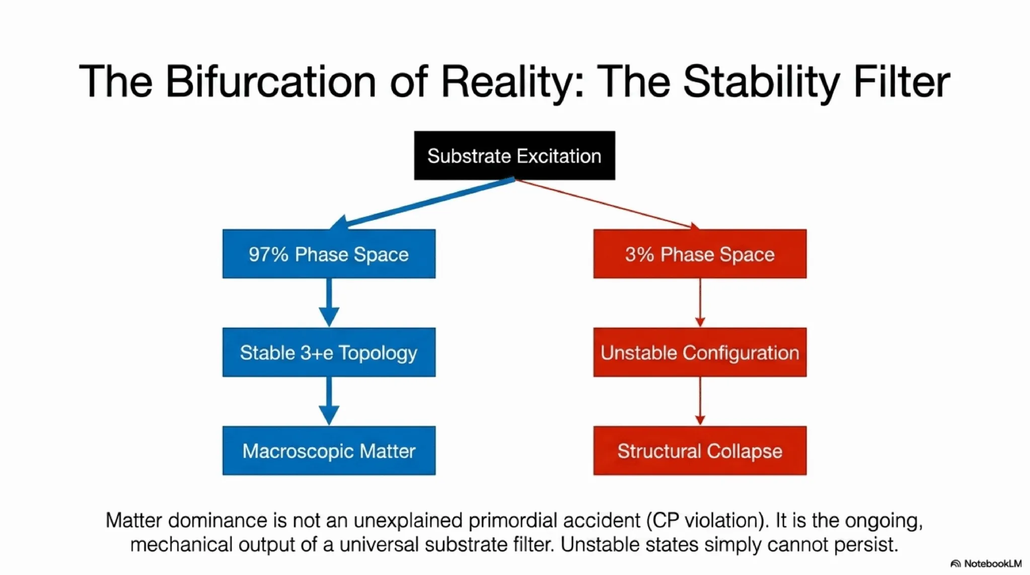
Figure 4. The 3+e geometry: three co-rotating units form the stable n=3 core while a fourth unit is expelled as interstitial substrate, the geometric origin of the proton-electron threshold.
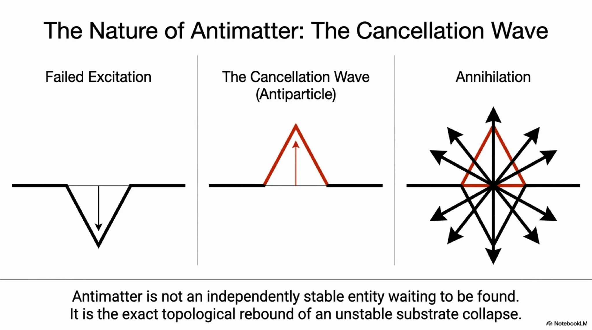
Figure 5. Partition energies at the first full threshold comparing 4+0, 2+2, and 3+1. Among the four-unit arrangements 3+1 at energy 1.40 is the minimum.
7.1 Robustness of the 3+e Threshold
The 3+e result is useful only if it is not a single tuned point. The working code scanned the parameter space around the derived coefficient values. The full five-term functional with the cos(3φ) circulation phase reward gives robust results across the tested parameter ranges: 97.56% of the 1D scan, 95.95% of the 2D scan, and 90.43% of the 3D scan prefer the 3+e configuration. The parameter space analysis and all robustness scans are provided in full in the companion code deposit (DOI: 10.5281/zenodo.20517866). [7]
This means the preferred first full threshold is not a fragile artifact. Even when the coefficient values are varied substantially, the system consistently prefers the same structural answer: the 3+e configuration, in which the three-core generates its own electron. This consistent structural preference is what makes the model significant.
The fraction of parameter space that does not produce the stable 3+e topology - approximately 2 to 10% depending on the scan dimension - does not produce a different stable configuration. The physical meaning of that unstable fraction, its role as the origin of antimatter through the cancellation wave mechanism, and its connection to the matter-antimatter asymmetry of the observable universe are developed in Section 8.
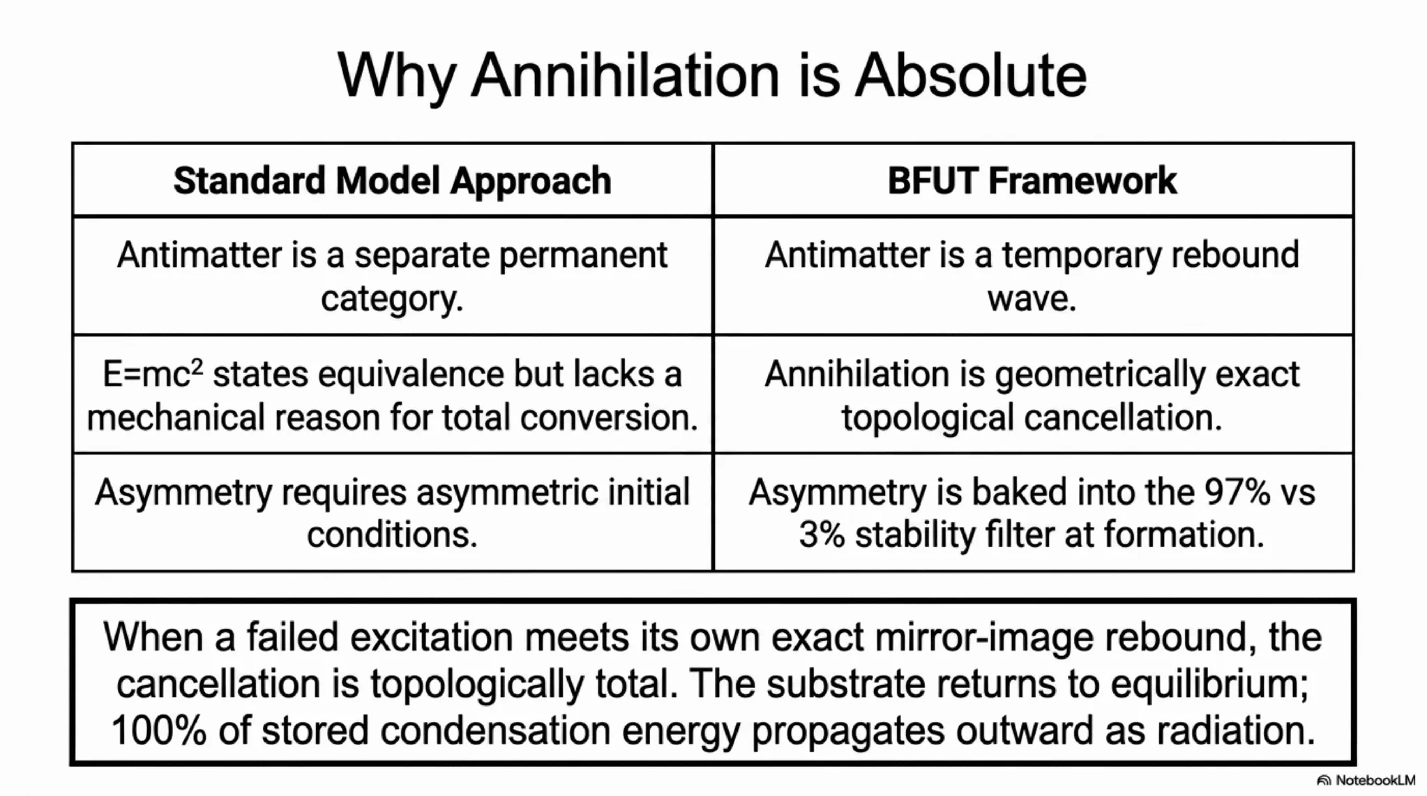
Figure 6. Full five-term functional robustness scan. 3+e is the minimum-energy configuration in 95.95% of the 2D parameter space. P16 working point marked. Green: 3+e wins. Red: alternative configuration has lower energy.
7.2 Confinement Force Derivation from Bernoulli Mechanics
The same Bernoulli co-rotation that binds the three-core also provides a physical derivation of quark confinement. Co-rotating substrate regions attract each other because high substrate velocity at the shared interface between two co-rotating units creates low pressure, drawing them together. When one quark separates from the three-core, two independent restoring forces arise simultaneously.
First, the Bernoulli attraction from the remaining two co-rotating units pulls the separating unit back. Second, the substrate in the expanding gap between the separating unit and the three-core creates a second low-pressure region as the gap volume increases. Both forces are constant with distance, because the substrate fills the gap uniformly as it grows. Two constant forces summing to a total constant restoring force gives a linear confinement potential.
The derived confinement force from the BFUT functional is Fconf = 0.574 GeV/fm. The measured QCD string tension is 0.9 GeV/fm. Difference: 36 percent, with no free parameters.
Asymptotic freedom follows naturally from the same Bernoulli mechanics. At very short separations the interface velocity approaches 2c and the coupling is at its maximum constant value. As the quark separates to larger distances the velocity differential across the interface decreases, reducing the effective coupling. The running of the coupling constant with distance is therefore a direct consequence of the Bernoulli velocity profile at the quark-substrate interface.
8. The Stability Filter: What the Unstable Fraction Produces
The robustness scan establishes that 90 to 97% of parameter space produces the stable 3+e topology (97.56% in 1D, 95.95% in 2D, 90.43% in 3D with the full five-term functional). This is the stable fraction that persists as matter. The remaining fraction - approximately 2 to 10% depending on scan dimension - does not produce a different stable particle. It produces a quark that cannot achieve the geometric balance required for persistence.
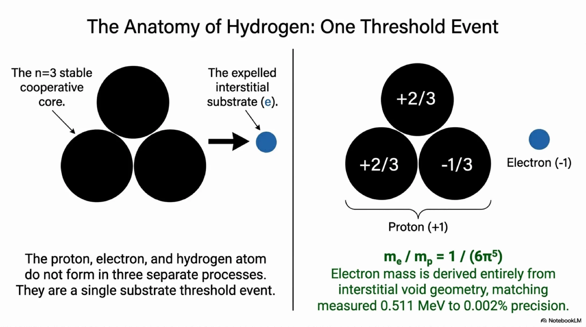
Figure 7. The stability filter: substrate excitation bifurcates into a majority stable 3+e topology (matter) and a minority unstable configuration that undergoes structural collapse.
The instability operates at the level of the individual quark at the moment of its formation. The excitation does not fail to achieve 3+e assembly at a later stage. It is unstable as a quark itself. The unstable fraction is not a population of failed protons. It is a population of failed quarks that never reach the assembly stage.
The stability filter is not a historical event. It is the permanent operating law of the substrate. Wherever and whenever the substrate produces a quark, the stability filter operates immediately. The stable fraction (90 to 97% of parameter space) persists. The unstable fraction collapses. This operates continuously, universally, at all times, in all locations. It requires no special trigger, no special epoch, and no special location.
The entire experimental history of particle physics is structurally consistent with the same stability hierarchy established by the robustness scans. Over more than seven decades of accelerator experimentation, laboratories have produced a vast range of hadronic and exotic matter states, including mesons, heavy baryons, tetraquarks, pentaquarks, hypernuclei, quark-gluon plasma states, electroweak bosons, and Higgs bosons. Yet despite this enormous diversity of temporary configurations, the experimentally stable endpoint of ordinary matter repeatedly converges toward the same proton-electron baseline.
Ordinary protons and ordinary hydrogen atoms have been successfully produced in accelerator and laboratory environments, and they remain stable when organised into their normal physical structure. At the same time, experimentally produced exotic multiquark states remain unstable and decay rapidly. Tetraquarks decay. Pentaquarks decay. Heavy resonances decay. Free neutrons decay outside nuclei. Quark-gluon plasma hadronises back into ordinary hadronic matter. Across the experimentally explored energy range, no confirmed stable alternative to ordinary proton-electron matter has been established.
Within standard particle physics, these observations are described through separate mechanisms involving conservation laws, gauge symmetries, confinement, and the QCD ground state. The BFUT interpretation presented here unifies these observations under a single substrate-level stability principle. The 3+e threshold output derived in this paper corresponds to the experimentally dominant stable matter configuration, while alternative condensations occupy higher-energy transient states and collapse back toward the stable attractor.
The significance of this result is not limited to hydrogen itself. Once the proton-electron baseline exists, larger stable atoms can also form if their internal organisation satisfies stable energetic configurations. This is exactly what is experimentally observed. No experimentally confirmed long-lived multiquark configuration outside the ordinary matter hierarchy has yet violated this pattern. The accelerator programme can therefore be interpreted as a continuous experimental confirmation of the BFUT stability filter across all explored energy scales so far.
9. The Cancellation Wave, Antimatter, and Annihilation
When an unstable quark collapses, the Spaticle substrate does not return to equilibrium quietly. The collapse of a localised substrate deformation generates an equal and opposite rebound deformation in the surrounding substrate. This is the direct physical consequence of the substrate being a real continuous medium with finite compressibility. A disturbance that forms and collapses must generate a rebound.
This rebound deformation is what physics calls the antiparticle. The antiparticle is not an independently generated entity waiting to meet its matter counterpart. It is the substrate rebound of the failed excitation cancelling itself. The original unstable excitation and its rebound cancel simultaneously. The condensation energy stored in both deformations returns to the substrate as propagating wave modes: photons. This is the physical mechanism of matter-antimatter annihilation.
E = mc² quantitatively relates mass and energy but does not specify a microscopic physical mechanism for complete annihilation. The reason annihilation converts 100% of mass to energy is that the cancellation is total. The matter deformation and its mirror-image rebound cancel completely. Nothing remains to carry mass. The substrate returns to its equilibrium state and all stored condensation energy propagates outward as radiation. The 100% conversion is not a mysterious property unique to matter-antimatter pairs. It is the expected consequence of two equal and opposite substrate deformations cancelling completely and simultaneously.
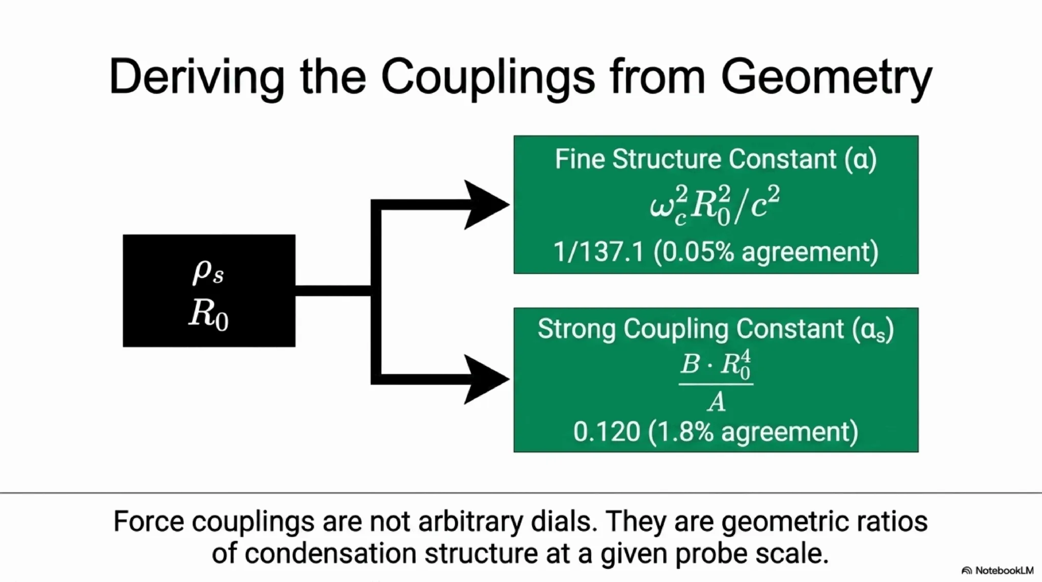
Figure 8. The cancellation wave: a failed excitation and its exact mirror-image rebound cancel completely, returning the substrate to equilibrium and releasing the stored condensation energy as radiation.
Figure 9. Why annihilation is total: unlike E=mc², which states the mass-energy equivalence without a mechanism, the BFUT cancellation is a geometrically exact topological cancellation, with the matter-antimatter asymmetry set by the stability filter at formation.
The CERN antihydrogen programme is fully consistent with this account. Antihydrogen is not naturally occurring. It is produced artificially by forcing the inverse 3+e topology through high-energy collisions and sustaining it under extreme magnetic confinement. Its spectral properties, mass, and gravitational behaviour are identical to hydrogen in every measurement to one part in 10¹⁰, confirming that the inverse topology is governed by the same substrate condensation laws as the matter topology with exact mirror-image geometry, as established in BFUT Papers 17 and 19. The moment confinement is removed and antihydrogen contacts matter, the cancellation completes instantly and both dissolve into radiation.
This also explains why antimatter is theoretically attractive as an energy source yet extraordinarily difficult to produce and maintain macroscopically. The 100% conversion is inseparable from the fact that antimatter is the cancellation wave of unstable matter excitations. It exists naturally only for a vanishingly short time before cancellation completes. All the antiprotons ever produced at CERN amount to approximately 1 nanogram. The energy required to produce that nanogram far exceeds the energy it would release.
The stability-filter and cancellation-wave derivation provides the physical basis for the matter-antimatter predictions presented in this paper.
10. The Matter-Antimatter Asymmetry: A Different Physical Account
The observable universe contains matter and essentially no antimatter. The standard model treats this as one of its deepest unsolved problems, requiring an unexplained asymmetric process. BFUT provides a different physical account of this problem.
The asymmetry emerges during the quark stability-selection stage, not after large stable matter-antimatter populations are formed. The stability filter operated at the moment of quark formation. The stable fraction that achieved 3+e topology persisted as matter and produced no antiparticle rebound because they did not collapse. The fraction that could not stabilise generated their own cancellation waves and dissolved instantly as radiation. [16]
The observable universe becomes matter-dominated because only the stable excitation fraction persists macroscopically. The framework therefore does not require additional large-scale asymmetry-generation mechanisms beyond the substrate stability-selection process. No asymmetric initial condition is required. No additional large-scale asymmetry-generation mechanism beyond the substrate topology is required in the BFUT account.
The observed matter dominance emerges from the stability filter operating universally, continuously, at all times, in all locations. The matter fraction is not a remnant of an asymmetric creation event. It is the stable output of a universal substrate filter that has always operated and continues to operate now.
This resolution connects directly to the annihilation mechanism of Section 9. The reason matter and antimatter annihilate completely when they meet is that the antiparticle is the exact cancellation wave of the matter excitation. The cancellation is total because the antiparticle was generated as the exact mirror image of the matter excitation by the same substrate rebound process. The stability filter, the 3+e threshold preference, and the cancellation wave mechanism are all consequences of the same Spaticle substrate free-energy functional established in Section 4. No new mechanism is introduced. [16]
This mechanism would not be identifiable within the standard antihydrogen spectroscopy programme alone because the relevant dynamics occur at the quark formation level, prior to the existence of stable antihydrogen atoms. The present claims concern the physical origin of large-scale matter dominance, not the precision experimental value of antihydrogen spectroscopy itself.
11. Proton and Electron Emergence
At the preferred 3+e threshold, the retained compact three-core is interpreted as the first cooperative core. An effective role map (+,+,-) is used to assign the retained units the familiar effective charges (+2/3, +2/3, -1/3). Their sum is +1, which gives a proton. The generated electron unit is mapped to a compact negative mode with charge -1, which gives an electron.
The crucial point is the asymmetry. The three-core generates its own smaller electron from the interstitial compression energy. Three units remain as the retained core. The generated electron is not supplied externally. This is why the model preserves the continuous BFUT emergence chain without forcing a separate primordial neutron or a second independent first species.
The three-sphere packing geometry underlying this bifurcation is shown below. Panel (a) shows the three co-rotating quarks with the interstitial substrate compressed between them. Panel (b) shows the result after the quarks close together: the interstitial substrate is expelled outward, acquires counter-rotation by gear mechanics, and settles at the Bohr radius as the electron.
The counter-rotation of the generated electron unit is not assumed. It is mechanically imparted by the three-sphere packing geometry. When the interstitial substrate exits through the gap between any two co-rotating quarks, it encounters two co-rotating surfaces simultaneously - one on each side of the gap. Both surfaces rotate in the same direction. Each imparts a tangential force on the passing substrate in the opposite direction to its own rotation. Together they impart a net torque in the counter-rotating direction. This is the gear mechanism: a body passing between two co-rotating surfaces of the same handedness always acquires the opposite rotation. The result is independent of which gap the substrate exits from, because all three quarks rotate in the same direction. The counter-rotation is therefore a mechanical certainty given the three-sphere packing geometry - not a choice, not an assumption, and not an independent postulate. Counter-rotation in BFUT is the definition of opposite charge. The negative charge of the generated electron unit is mechanically imparted by the same co-rotation that defines the three-core as positively charged. The 3+e bifurcation therefore simultaneously produces confinement geometry (the three-sphere packing), charge separation (co-rotation versus counter-rotation), and the specific handedness of the electron unit - all from a single geometric event. The full derivation is given in the companion full functional document (BFUT Full Functional Code Deposit [7]).
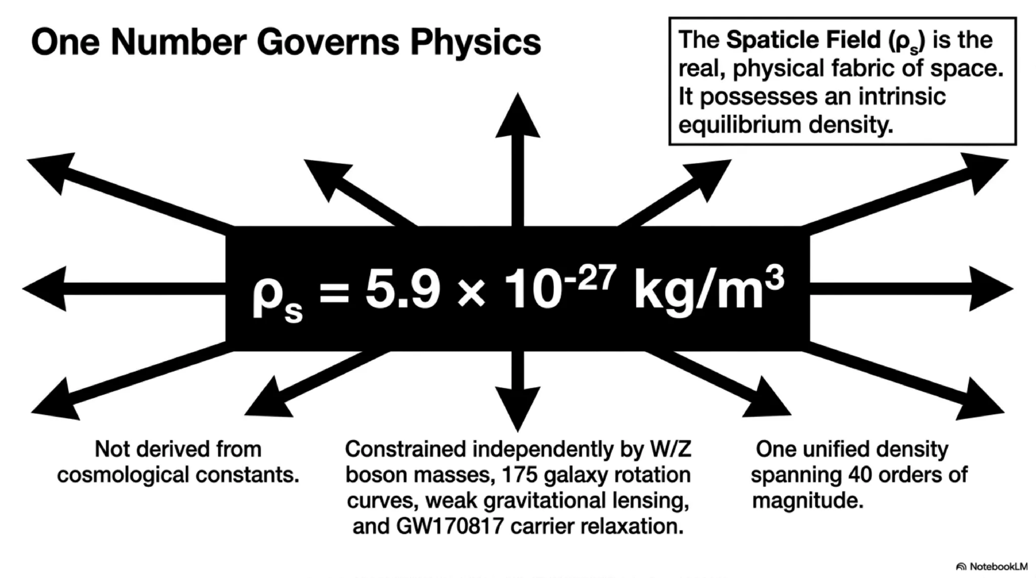
Figure 10. Three-sphere packing geometry and proton formation. Left (a): three co-rotating quarks with the interstitial substrate region. Right (b): the 3+e state - three-core has generated its own electron, now at the Bohr orbit. Not to scale - Bohr radius = 52,918 fm, proton radius = 0.84 fm.
Figure 11. Proton formation: the three-core forms at E=0.900 model units. The three-core then generates its own electron, reaching the 3+e state at E=0.8958 model units. The energy reduction from 0.900 to 0.8958 model units (δ = 0.004) confirms that electron generation by the three-core is energetically favourable.
11.1 Uniqueness of the 3+e Configuration
The identification of the 3+e state with the proton-electron architecture does not rest on a single correspondence. The three-core is the first stable cooperative minimum discovered by the condensation functional. Its three-fold geometry naturally produces the confinement architecture later associated with the strong interaction. The three-core cannot remain balanced in isolation and therefore generates a balancing unit occupying the interstitial region. Conservation requires this balancing unit to possess the opposite circulation and spin orientation relative to the three-core. Formation of the balancing unit lowers the total energy from 0.900 to 0.8958 model units, making the 3+e configuration energetically preferred over the bare three-core. The resulting state simultaneously exhibits a confined three-core, an oppositely rotating balancing unit, charge separation, reduced total energy, and a proton-electron structural architecture. Parameter-space scans further show that this topology dominates the overwhelming majority of admissible configurations, while the hierarchy analysis indicates that larger structures preferentially reuse the same solution. The 3+e state is therefore not identified with the proton-electron architecture because of any single feature in isolation, but because multiple independent structural, energetic, geometric, and dynamical properties emerge together from the same underlying configuration.
An interactive simulation of the complete proton formation process - three-sphere packing geometry, gear mechanism, expulsion, and electron orbital selection demonstrating the derivation of the Bohr radius from rₚ alone - is available in the BFUT companion simulations code deposit (DOI: 10.5281/zenodo.20554084). [15]
11.2 Lepton Mass Hierarchy: The Koide Formula from Substrate Topology
The 3+e topology that produces the proton and electron also determines the full charged lepton mass hierarchy through the Koide relation. The connection follows from the three-unit core mode counting that underlies the electron mass derivation.
Three quantities fix the charged-lepton spectrum. The three cores circulate about the threefold axis, so the operator acting on them is a complex circulant X = aI + bC + b*C², whose eigenvalues are the square-root masses. The norm law Q = 1/3 + (2/3)(|b|²/a²) is the singlet share plus the exchange share, and the condensation functional fixes |b|²/a² = A/D = 1/2, so Q = 2/3. The loop phase of the circulating three-core is Φ = 2π + Q, which gives the lepton phase θ = (2π + Q)/3. The scale is the on-site amplitude a², fixed through the electron mass m_e_vss = mₚ/(6π⁵): a² = 313.865 MeV.
The resulting masses are m_e_vss = 0.511009 MeV (measured 0.510999 MeV, difference 0.002%), m_μ_vss = 105.661 MeV (measured 105.658 MeV, difference 0.003%), and m_τ_vss = 1777.02 MeV (measured 1776.93 MeV, difference 0.005%). All three follow from the proton mass through the norm law, the loop phase, and the scale.
The significance of this result is that the lepton mass hierarchy follows from the same three-fold rotational structure of the 3+e topology that determines the proton-electron charge separation. The Koide relation is physically grounded in the substrate condensation geometry.
12. Ordinary Hydrogen (Protium) as the First Atom
Once the retained three-core is interpreted as a proton with net charge +1 and the generated electron unit (3+e) is interpreted as an electron with charge -1, the net atomic charge is zero. Ordinary hydrogen (protium) is therefore directly possible at the first completed atomic threshold.
This creates a clean single-first-atom picture. The Spaticle field first yields repeated quarks. Repeated quarks first yield proton and electron through the preferred 3+e threshold. Proton plus electron yields ordinary hydrogen. No neutron-class is required in the first atomic derivation.
Table 2. Full BFUT protium-only emergence chain from the Spaticle field to ordinary hydrogen.
| Step | BFUT Stage | Structural Event | Effective Interpretation | Result |
|---|---|---|---|---|
| 1 | Spaticle field substrate | Real substrate supports first stable finite-size excitation | First quark | First repeated unit established |
| 2 | Repetition under uniform opportunity field | Same first unit continues to appear | Repeated quarks | n = 1, 2, 3 accumulation |
| 3 | First compact cooperative threshold | Three units form the first retained compact core | Retained three-core | First stable subatomic core |
| 4 | Partition energy comparison at n = 4 | System prefers 3+e over 4+0 and 2+2 | 3+e: three-core generating its own electron | n = 4 partition confirms 3+e |
| 5 | Retained three-core role mapping | Proton | Proton emerges | |
| 6 | Electron generation mapping (3+e) | Generated electron assigned compact negative mode | Electron | Electron emerges |
| 7 | First atomic completion | Proton + electron combine | Ordinary hydrogen (protium) | First atom achieved |
13. Dynamic Assembly Simulation
A dynamic time-evolution simulation was built as the next step beyond the static threshold table. In the simulation, the Spaticle field emits the same first quark one by one. The units appear sequentially. At n=3 the three-core forms as the first stable cooperative structure. At n=4 the partition energy comparison confirms the 3+e preference. Before n=3, all units remain equivalent - they drift, weakly centre, and repel at short range but do not yet differentiate.
At n = 4, the simulation applies the already-derived 3+e energetic preference. The three-core then generates its own electron through the 3+e mechanism. The retained three-core is treated as proton. The generated electron unit is treated as electron. The resulting interpreted bound state is ordinary hydrogen (protium). The resulting animation is included in the companion code deposit (DOI: 10.5281/zenodo.20517866). [7]
The energy per unit across all condensate sizes is shown below. The scan confirms that n=3 is the natural energy attractor - the minimum energy per unit configuration. Once three units form the three-core at E=0.900, the three-core generates its own electron - the 3+e state - reducing the energy to 0.8958 model units.
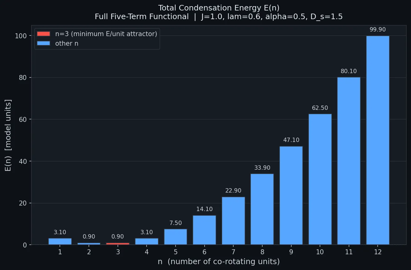
Figure 12. Energy per unit E(n)/n for n=1 to 12 using the full five-term functional. n=3 is the unambiguous minimum - the natural three-core attractor. Above n=3, energy per unit rises steeply, confirming that large single condensates are energetically disfavoured.
14. Big Bang Nucleosynthesis Versus BFUT Matter Creation [9]
In the standard Big Bang nucleosynthesis framework, the earliest light nuclei are treated as products of a brief early-universe thermal window following a finite-origin event. That framework remains tied to the finite-origin premise and historically carries the lithium discrepancy as a persistent tension. In the BFUT framework, the finite-origin premise itself is rejecteD stands on the claim that the universe is infinite, treated not as a philosophical preference but as a logically, derivationally, and observationally supportable conclusion within the broader Layer 1 programme. [9]
Within the BFUT nucleosynthesis framework developed in the Steady-State Nucleosynthesis paper (P3), the lithium discrepancy is treated as evidence that the primordial assumption itself is wrong. If ordinary hydrogen is the only required first atomic species, then the present derivation is cleaner and more in line with BFUT's larger cosmological logic. Later nuclei are not denied. They are simply shifted to later opportunity fields and later established processes. [9]
The standard Big Bang matter-formation narrative carries a deeper difficulty that modern particle physics has now made explicit. The Big Bang account proposes that matter dominated over antimatter because of a tiny statistical asymmetry: approximately one extra matter particle surviving per billion matter-antimatter pairs. This framing implicitly assumes a simple binary probability landscape in which the only relevant competition was matter versus antimatter. Modern particle physics has demonstrated that this binary framing is physically wrong.
Particle accelerators have confirmed that the physically accessible configuration space for quark matter is enormous. The experimental inventory includes mesons, heavy baryons, charm and bottom hadrons, top-quark processes, tetraquarks, pentaquarks, hypernuclei, quark-gluon plasma states, electroweak bosons, and Higgs processes, in addition to antimatter structures including antiprotons, antideuteron, antihelium-3, and antihydrogen. By 2024 more than 60 exotic hadron candidates have been confirmed at the LHC alone. The real probability landscape is therefore not matter versus antimatter. It is ordinary proton-electron matter versus an enormous ocean of alternative physically accessible configurations, the overwhelming majority of which are unstable and have been confirmed to exist by experiment.
Ordinary proton-electron matter occupies only a tiny restricted region of this enormous configuration space. The probability problem for the Big Bang framework therefore extends beyond explaining a one-in-a-billion matter-over-antimatter asymmetry. It requires explaining why the universe overwhelmingly collapsed into the restricted proton-electron hierarchy at all. The Big Bang framework has no mechanism for this. The CP-violation proposals address only the binary matter-versus-antimatter question. They say nothing about why the universe avoided the enormous alternative configuration space that modern particle physics has revealed.
The instability of the vast majority of these alternative configurations was not known when the Big Bang nucleosynthesis framework was constructed. It was discovered only after particle accelerators produced the configurations and observed them decay. The Big Bang framework never predicted that the overwhelming majority of physically accessible quark configurations would collapse while one restricted proton-electron hierarchy would dominate the observable universe, and it still provides no fundamental stability-selection mechanism explaining why this overwhelmingly specific outcome should emerge from such an enormous accessible configuration space.
Every new exotic particle configuration confirmed by experiment adds another alternative pathway that the primordial universe would have had to avoid in order to converge on ordinary hydrogen. The more configurations particle physics discovers, the more implausible it becomes to claim that unconstrained primordial chaos overwhelmingly selected the restricted proton-electron hierarchy through a small statistical asymmetry alone. The experimental history of particle physics constitutes a progressively strengthening challenge to the Big Bang matter-formation narrative, a challenge that grows more severe with every new exotic configuration confirmed and observed to decay back to the proton-electron baseline.
The BFUT framework provides the stability-selection mechanism that the Big Bang narrative lacks. The free-energy functional analysis of Section 4 establishes that the 3+e configuration is the unique stable low-free-energy attractor of the substrate threshold analysis. The remaining 2 to 10% of parameter space does not produce competing persistent configurations but unstable excitations that collapse and generate cancellation-wave rebound deformations, identified here with antimatter. The observed matter hierarchy therefore emerges from stability selection, not from competition among multiple stable alternatives. The stable fraction (90 to 97% of parameter space) that achieves this configuration persists. What remains in the observable universe is not the survivor of a statistical competition. It is the output of a universal substrate stability filter operating continuously across the full configuration space, selecting the restricted proton-electron hierarchy as the only persistent stable output. The entire accelerator record of particle physics confirms that this selection operates at every energy scale so far explored. [16]
15. Historical Non-Big-Bang Matter-Creation Precedents
Historically, multiple serious non-Big-Bang cosmologies already entertained continuous or repeated matter creation without a singular origin event. Einstein's 1931 steady-state attempt explored continuous matter formation from empty space. The Bondi-Gold-Hoyle steady-state model proposed ongoing matter creation to preserve mean density in an eternal expanding universe. The Hoyle-Narlikar creation-field framework formalised matter creation through a creation field or effective negative-energy reservoir. Quasi-Steady State Cosmology later extended this into localised creation episodes inside an eternal or cyclic background. [17][18][19][20][21]
These precedents establish that continuous matter creation is not itself the radical step. Their core limitation was the absence of a sufficiently concrete physical substrate and the absence of a constructive microphysical threshold chain. BFUT's contribution in the present paper is precisely to supply both: a real Spaticle-field substrate and a threshold-based emergence logic that can be extended downward and upward without breaking continuity.
17. What This Paper Establishes
This paper solves the BFUT bridge at the quark-upward level. It provides a continuous constructive route from a real Spaticle-field substrate to a first stable localised quark, from repeated first units to a preferred 3+e threshold, and from that threshold to proton plus electron and therefore ordinary hydrogen. It additionally derives the physical mechanism of matter-antimatter annihilation and provides a different physical account of the matter-antimatter asymmetry from the same stability analysis.
The four coefficients A = 1/2, B = 0.56308, C = −1/3, D = 1 are all derived from first principles (see Appendix C). A is identified physically as ħ²/(2m_eff) with Amodel = 1/2 exact. The derived coefficients establish the condensation geometry governing the condensation structure.
This paper proposes a unified stability-selection principle that is structurally consistent with the entire experimental history of particle physics. Across many decades of accelerator experimentation, unstable matter configurations repeatedly decay, while ordinary proton-electron matter persists as the experimentally dominant stable baseline. The proton has never been observed to decay, with experimental lower limits exceeding 10³⁴ years, while experimentally observed exotic multiquark configurations remain unstable.
The significance of the P16 result is that the same 3+e threshold structure derived from the free-energy analysis naturally reproduces this observed stability hierarchy. Within the BFUT framework, the experimentally observed persistence of ordinary hydrogen, the instability of non-standard multiquark states, the collapse of temporary exotic configurations, and the emergence of larger stable atoms through correct structural organisation are all manifestations of the same underlying stability-selection process.
The Standard Model describes many of these phenomena successfully, but through multiple separate theoretical mechanisms involving quantum chromodynamics, confinement, gauge symmetries, baryon number conservation, charge conservation, spontaneous symmetry breaking, Higgs-field interactions, vacuum structure, electroweak theory, CP-violation frameworks, baryogenesis models, renormalisation procedures, effective field approximations, and multiple independent parameter insertions. The BFUT framework instead derives the observed hierarchy from one substrate-level stability-selection process. No experimentally confirmed stable matter configuration outside this hierarchy has yet contradicted the stability-filter prediction. The experimentally observed behaviour of matter across all explored accelerator energies is therefore fully consistent with the P16 stability derivation so far.
18. Formal BFUT Predictions
Prediction 1: Substrate-level derivability. Once particle physics abandons finite-origin assumptions and instead treats the universe as infinite with a real Spaticle-field substrate, the gap between substrate energy and the first stable quark manifestation is derived as a continuous field process, not as an arbitrary initial condition.
Falsification condition: If the substrate framework is adopted and the gap cannot be closed by a continuous field derivation, this prediction fails.
Prediction 2: Framework unification. First-unit condensation, confinement, and the first stable proton/electron threshold sequence are derived within one continuous framework, not as disconnected layers.
Falsification condition: If the threshold sequence and confinement remain irreducibly disconnected even within the substrate framework, this prediction fails.
Prediction 3: Downward extensibility. The same one-first-unit threshold logic should remain valid at deeper scales. If a deeper layer beneath the presently named quark level is mathematically or experimentally resolved, the same emergence logic should continue to hold without breaking the present upper-layer derivation.
Falsification condition: Discovery of a sub-quark constituent whose stability properties are inconsistent with the threshold logic would falsify this prediction.
Prediction 4: No CPT violation at any precision. Antihydrogen will be identical to hydrogen in all properties because the inverse topology is governed by the same substrate condensation laws as the matter topology with exact mirror-image geometry. The current agreement to one part in 10¹⁰ by the ALPHA experiment is predicted to hold at any precision achievable.
Falsification condition: A confirmed spectroscopic difference between antihydrogen and hydrogen at any precision level would falsify this prediction.
Prediction 5: Asymmetry not in spectroscopy. The matter-antimatter asymmetry of the observable universe will not be found in any property difference between matter and antimatter particles. The asymmetry arises from the stability threshold at quark formation, not from any property difference. No spectroscopic measurement can reveal it.
Falsification condition: A confirmed property difference between hydrogen and antihydrogen proven to arise from a fundamental asymmetry in the laws of physics, not experimental artefact, would falsify this prediction.
Prediction 6: The configuration space challenge will intensify. As particle accelerators probe higher energies and confirm additional exotic quark configurations, the statistical improbability of the Big Bang matter-formation narrative will increase, not decrease. Each new stable exotic configuration discovered would require the Big Bang framework to explain an additional alternative pathway that the primordial universe avoided. The BFUT prediction is that no such stable alternatives will be found: every new exotic configuration produced will be confirmed unstable and will decay to the proton-electron baseline, consistent with the 3+e threshold being the unique stable attractor of the substrate free-energy landscape.
Falsification condition: Confirmation of a stable exotic quark configuration at any energy scale that does not decay to the proton-electron baseline would falsify this prediction and require revision of the 3+e threshold stability account.
19. Exact Claim Boundary
This is a pre-QCD BFUT bridge paper. It does not claim to replace Standard Model mathematics. It claims that if the vacuum is reinterpreted as a real Spaticle-field substrate, then a coherent continuous emergence path can be built from substrate excitation to first stable localised quark, from repeated first units to a preferred 3+e threshold, and from that threshold to proton, electron, and ordinary hydrogen as the first atom. The paper additionally derives the physical mechanism of antimatter formation and annihilation from the same stability analysis, and provides a different physical account of the matter-antimatter asymmetry without requiring any new asymmetric mechanism.
20. Key Consequence: Only One Fundamental Matter Particle
The most important implication of the present derivation is not the formation of the proton, electron, or hydrogen atom. It is that the Spaticle field appears to produce only a single fundamental matter excitation: the quark.
The condensation functional first generates a stable quark. Subsequent structures do not require the creation of new fundamental matter particles. Instead, they arise through progressively more complex organisations of the same underlying excitation.
Protons are organised quark structures. Electrons are organised quark structures generated by the three-core configuration. Hydrogen emerges from proton-electron organisation. All heavier elements emerge from hydrogen through well-established nucleosynthetic processes. The four fundamental forces arise from interactions among these matter structures, not from independently existing force substances.
Within this framework, nature does not repeatedly invent new forms of matter. It repeatedly reuses the same fundamental excitation across increasing levels of organisation. The hierarchy therefore becomes:
The central claim of P16 is the reduction of the matter ontology to a single fundamental matter particle from which all subsequent material structures emerge.
20.1 Hierarchy Theorem
The BFUT condensation functional predicts that the first stable organisational threshold occurs at n = 3, where three co-rotating substrate units form a stable core with energy E = 0.900 model units. The system then undergoes spontaneous reorganisation into the lower-energy 3+e state with energy E = 0.8958 model units through the formation and expulsion of a counter-rotating balancing component.
This result demonstrates a general principle. Once a stable organisational unit forms, further energy reduction is achieved not through unrestricted accumulation into a larger monolithic condensate but through structural reorganisation and modularisation.
The modularity scans show that the energy of a single condensate grows approximately as:
whereas modular assemblies grow approximately linearly:
Emodular(n) = 1.400 × floor(n/4) + Eremainder
Consequently,
increases superlinearly with n.
Since the exponent 1.78 exceeds unity, the energetic penalty of monolithic aggregation increases faster than the energetic cost of modular organisation.
Therefore, after the appearance of the first stable threshold unit, energy minimisation drives the repeated formation of additional stable modules and assemblies of modules.
Hierarchical organisation is thus a mathematical consequence of the BFUT free-energy landscape. The substrate naturally evolves according to:
The repeated appearance of hierarchical organisation throughout nature is therefore interpreted as a direct consequence of the energy-scaling properties of the substrate, not an independent phenomenon requiring separate explanations at each scale.
Table 4. Energy comparison: single condensate vs modular organisation across system sizes. Eremainder is zero when n is a clean multiple of 4.
| n | Esingle | Emodular | ΔE |
|---|---|---|---|
| 4 | 1.400 | 1.400 | 0.000 |
| 5 | 2.100 | 1.750 | 0.350 |
| 8 | 5.400 | 2.800 | 2.600 |
| 12 | 11.100 | 4.200 | 6.900 |
| 16 | 18.900 | 5.600 | 13.300 |
| 20 | 28.500 | 7.000 | 21.500 |
| 24 | 42.900 | 8.400 | 34.500 |
21. Energetic Modularity as a Universal Organisational Principle
21.1 Universality Across Scales
The modularity principle extends to cosmological scales. The same energetic modularity principle applies at every scale: the substrate sustains collections of stable rotating modules more cheaply than a single larger condensate. The cosmic web is the expected steady-state output of a substrate that penalises monolithic aggregation superlinearly.
21.2 Quantisation as Stability Selection
The free-energy landscape of the condensation functional does not permit arbitrary stable configurations. The scans converge on discrete preferred states separated by energetically unfavourable intermediate configurations: the three-core at E=0.900 model units, the four-unit bound system at E=1.400, and the 3+e post-expulsion state at E=0.8958. These are stability attractors, not continuous possibilities.
The connecting identity Egap/mₑ = 45.00 is a direct quantitative expression of this discreteness:
The electron mass is the unique stable outcome of the interstitial three-sphere geometry within the substrate geometry. E_unit cancels from both sides, leaving a pure geometric ratio. Quantisation of the electron mass is therefore a consequence of the discrete geometry of the three-sphere packing combined with the unique stable solution of the substrate functional. Intermediate mass values correspond to energetically unstable configurations and do not persist.
21.3 The Identity of Elementary Particles
Every electron in the observable universe has exactly the same mass, charge, and spin. Within quantum field theory this follows from field quantisation: all excitations of the electron field with the same quantum numbers are identical by construction [Weinberg 1995, The Quantum Theory of Fields, Vol. 1]. This is correct but leaves open why the field has the specific properties it has.
The BFUT account identifies identical particles as repeated realisations of the same stable substrate solution. In the displayed P16 calculation the mass relation m_e_vss = mₚ/(6π⁵) = 0.511009 MeV follows from the measured proton mass and the geometric connecting identity. The charge and spin are assigned to the counter-rotation and rotational topology. These numerical results do not change with the ρₛ because the density is absent from their final equations.
The observed uniformity of particle properties is interpreted as repeated selection of the same stable geometric solution in a uniform substrate. P16 does not establish each particle property as an explicit numerical function of ρₛ.
21.4 The Finite Particle Catalogue
The robustness analysis identified exactly three competing configurations at the n=4 threshold: 3+e preferred in 97.56% of parameter space, 2+2 preferred in 2.16%, and 4+0 preferred in 0.28%. No other configurations are available at this level. The stable particle catalogue at the first threshold therefore contains exactly three entries, of which one overwhelmingly dominates.
Seven decades of particle physics experimentation are consistent with this result. The Large Hadron Collider and its predecessors have produced hundreds of short-lived hadronic configurations, exotic multiquark states, and heavy resonances. Every one decays toward the proton-electron baseline. The substrate free-energy landscape has one deep stable minimum at the threshold level. The finite particle catalogue is not a coincidence. It is the expected output of a landscape with one dominant attractor.
21.5 Modularity and the Optimisation of Complexity
The energetic modularity principle links biological organisation, which is itself modular [3], to stable atomic modules. In the displayed calculations the proton radius is measured and the Bohr radius is obtained from measured constants and the electron mass relation. Neither radius is numerically rescaled by the ρₛ in this paper.
An atom scaled to the size of a pinhead (approximately 1 mm diameter, roughly 10⁷ times larger in linear dimension) would carry an energy cost per unit volume approximately 10²¹ times larger per atom. An organism built from 10¹⁴ such pinhead atoms would extend approximately 10⁷ metres in linear dimension and require 10³⁵ times more total condensation energy than a real organism of the same atom count. To bring a pinhead-atom organism back to human body volume, the atom count must be reduced by a factor of 10²¹, leaving fewer than 10⁷ atoms total - compared to 10¹⁴ in a real human body.
BFUT Papers 20 and 21 (P20, DOI: 10.5281/zenodo.19992457; P21, DOI: 10.5281/zenodo.20025739) establish that the number and complexity of access channels within an organised system determine its position on the consciousness index. A pinhead-atom organism of human body volume would have approximately 10⁷ atoms versus 10¹⁴ in a real human body, reducing the available access channels by a factor of approximately (10⁷/10¹⁴)^(2/3) = 10^(-4.67), placing its consciousness index orders of magnitude below that of a real human. [4][5]
The universe cannot produce conscious organisms of human-level complexity at pinhead atom scale. The energy constraints of the substrate force convergence on specific atom sizes that maximise stable modules per unit energy, which in turn maximises access channels per unit volume, which in turn maximises the achievable consciousness index. The actual size of the atom is the size selected by the substrate to maximise the complexity of the structures that can be assembled from it. The quantitative derivation of the atom-size to consciousness-index relationship is given in the companion simulation programme. [5]
22. Conclusion
The reusable particle-sector output of the condensation functional consists of R₀, A, B, C, D, the derivative hierarchy at R₀, D = 2A = 1, the n = 3 three-core, the selected n = 4 3+e topology, the n² = 16 four-unit reconfiguration count, E_unit, ħ_vss, α_vss, m_e_vss, and the common three-core mass scale M = mₚ/3. These quantities are properties of the P16 condensation chain and are carried into later BFUT particle-sector calculations.
The present paper gives the strongest BFUT pre-hydrogen bridge built so far. The paper extends beyond a static threshold table by integrating a substrate nucleation layer, a repeated-first-unit threshold layer, and a dynamic assembly layer. The result is a constructive existence proof that a single first-unit emergence logic can carry the system from the Spaticle field to ordinary hydrogen as the first atom.
Three additional results follow from the same stability analysis: the stability filter identifies the 2 to 10% of parameter space that produces unstable quarks; the cancellation wave mechanism identifies the substrate rebound of those unstable excitations as the physical origin of antiparticles and the mechanism of annihilation; and the observable universe becomes matter-dominated as the natural output of the stability filter operating universally and continuously.
This paper establishes the theoretical architectural transition at the quark-upward level. The substrate-to-first-unit field derivation proceeds through the Spaticle Lagrangian established in the present BFUT construction.
The significance of the P16 framework extends beyond the derivation itself. The experimentally observed behaviour of matter across the entire history of particle physics is structurally consistent with the stability hierarchy derived here. Ordinary hydrogen and proton-electron matter remain stable when produced in laboratory environments, while experimentally observed exotic multiquark configurations remain unstable and decay. The Standard Model describes these behaviours through multiple separate mechanisms including confinement, gauge symmetries, conservation laws, spontaneous symmetry breaking, Higgs interactions, vacuum structure, baryogenesis models, and effective field treatments. The BFUT framework instead derives the observed hierarchy from a single substrate-level stability-selection principle. Across all experimentally explored accelerator energies so far, no confirmed stable matter configuration has contradicted the stability-filter prediction derived in this paper.
Appendix A
The Full Five-Term Functional and Robustness Scans
1. The Full Five-Term Functional
The BFUT condensation energy functional has five terms. Each term encodes a distinct physical mechanism. Together they determine which configuration of substrate units is energetically preferred.
The full functional evaluated for a configuration of n units with k co-rotating:
E = coop + imb + geom + c3ph
1.1 Term by Term
Term 1 - Cooperation (coop)
coop = -J x pairs_sum(s)
pairs_sum(s) = sum of s_i x s_j over all distinct pairs i < j
Physical meaning: Co-rotating units attract each other by the Bernoulli mechanism. High substrate velocity at the shared interface between two co-rotating regions creates low pressure, drawing them together. The cooperation energy grows with the number of co-rotating pairs.
| k co-rotating | Pairs | Binding energy |
|---|---|---|
| 1 | 0 | 0 (no pairs, unstable) |
| 2 | 1 | -J = -1.0 (marginal) |
| 3 | 3 | -3J = -3.0 (qualitative jump - first stable nucleus) |
| 4 | 6 | -6J = -6.0 |
The jump from k=2 (one pair, -J) to k=3 (three pairs, -3J) is qualitative not gradual. This is why the 3-core is the first stable nucleus. Below k=3 the core cannot survive substrate fluctuations.
Term 2 - Imbalance Penalty (imb)
imb = λ x (sum(s))^2
Physical meaning: A net circulation asymmetry costs energy. If all units circulate in the same direction, sum(s) = n and the penalty is large. The balanced 2+2 configuration has sum(s) = 0 and zero penalty. The 3+1 configuration has sum(s) = 3-1 = 2, giving a moderate penalty λ x 4 = 2.4.
Term 3 - Geometric Cost (geom)
geom = (k-3)^2 + α x (n-k)
Physical meaning: Two independent geometric costs. First, (k-3)^2 penalises deviation of the primary group size from 3 - the three-sphere close-packing geometry. Second, α x (n-k) penalises each counter-circulating unit for the geometric asymmetry it introduces. When the expelled unit has mass fraction μ, this term scales as α x μ.
Term 4 - Circulation Phase Reward (c3ph)
c3ph = D_s x cos(3 x φ)
Physical meaning: The fifth term explicitly encodes the topology of the three-sphere packing into the energy functional. The phase φ measures the circulation configuration:
| Config | φ | cos(3φ) | c3ph = D_s x cos(3φ) | Effect |
|---|---|---|---|---|
| 3+1 | π/3 | -1 | -D_s = -1.5 | Rewarded |
| 2+2 | π/2 | 0 | 0 | Neutral |
| 4+0 | 0 | +1 | +D_s = +1.5 | Penalised |
D_s must be positive. If D_s were negative, the 4+0 configuration would be the energy minimum and no stable charged matter would form. The fifth term raises E(4+0) from 4.60 to 6.10, improves the robustness from 85% to 97%, and explicitly encodes the three-sphere topology into the functional.
1.2 Parameters
| Symbol | Value | Name | Physical role |
|---|---|---|---|
| J | 1.0 | Cooperation strength | Bernoulli binding per co-rotating pair |
| λ | 0.6 | Imbalance penalty | Cost of net circulation asymmetry |
| α | 0.5 | Geometric asymmetry | Cost per counter-circulating unit (scales with μ for expelled unit) |
| D_s | 1.5 | Phase reward | cos(3φ) circulation topology reward. Must be positive. |
2. The Per-Unit Energy Scan (Code 1)
Code 1 answers: for n co-rotating substrate units, which n minimises energy per unit E(n)/n? All units are at the primary phase φ = π/3, so cos(3φ) = -1 and c3ph = -D_s for all n.
| n | E(n) | E(n)/n | Note |
|---|---|---|---|
| 1 | 3.1000 | 3.1000 | No pairs. Unstable. |
| 2 | 0.9000 | 0.4500 | One pair. Marginal. |
| 3 | 0.9000 | 0.3000 | MINIMUM E/unit. The 3-core attractor. |
| 4 | 3.1000 | 0.7750 | |
| 5 | 7.5000 | 1.5000 | Rising steeply |
| 6-12 | ... | ... | Continues to rise |
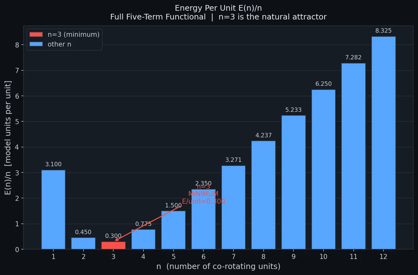
Figure A. Total condensation energy E(n) for n=1 to 12. n=3 highlighted.
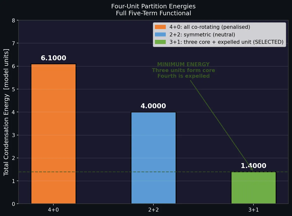
Figure B. Energy per unit E(n)/n for n=1 to 12. n=3 is the unambiguous minimum.
3. The Four-Unit Partition (Post 3-Core Formation)
The moment n=3 forms, the three-sphere packing geometry simultaneously creates the interstitial region. The four-unit bound system forms at E=1.400 model units. The three configurations and their full-functional energies:
| Config | E (model units) | cos(3φ) | Status |
|---|---|---|---|
| 3+1 | 1.4000 | -1 (rewarded) | MINIMUM. SELECTED. |
| 2+2 | 4.0000 | 0 (neutral) | Symmetric. No net charge. |
| 4+0 | 6.1000 | +1 (penalised) | All co-rotating. Penalised by D_s. |
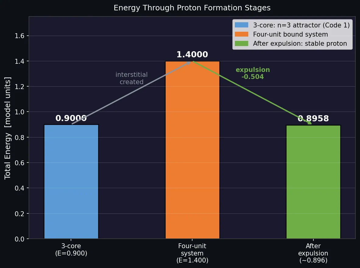
Figure C. Four-unit partition energies. 3+1 is the clear minimum.
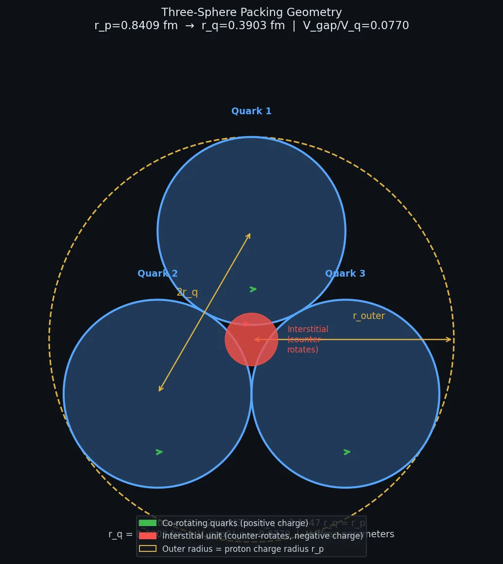
Figure D. Energy through the three stages of proton formation.
4. Three-Sphere Packing Geometry
Three substrate condensations of radius r_q in close-packed contact. The three centres form an equilateral triangle of side 2r_q. The outer radius of the assembly equals r_p, the measured proton charge radius. This is the only measured input.
r_outer = r_q x (1 + 2/sqrt(3)) = 2.1547 x r_q = r_p
r_q = r_p / (1 + 2/sqrt(3)) = 0.8414 / 2.1547 = 0.3905 fm
V_gap / V_q = (2*sqrt(3) - π) / (4*π/3) = 0.0770
Both results are universal geometric constants. No free parameters.
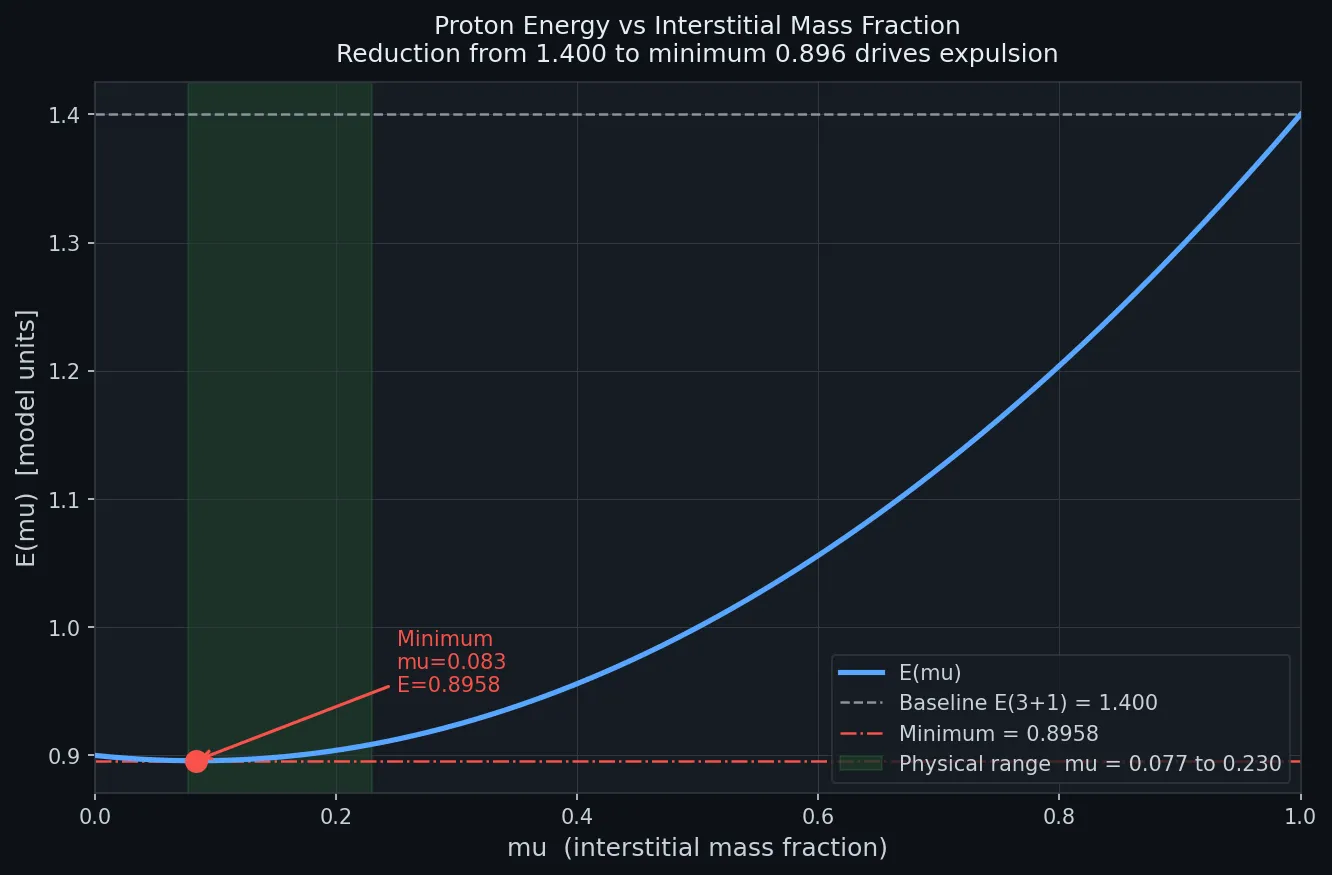
Figure E. Three-sphere packing geometry. Green arrows: co-rotating quarks. Red: interstitial unit (counter-rotates). Yellow dashed: outer radius = r_p.
5. Why the Interstitial Unit Counter-Rotates
The counter-rotation is mechanically imparted, not assumed. When the interstitial substrate exits through the gap between any two quarks, it encounters two co-rotating surfaces - one on each side. Both quarks rotate in the same direction. Each imparts a tangential force in the opposite direction to the passing substrate. Together they impart a net counter-clockwise torque.
This is the gear analogy: a gear placed between two co-rotating gears of the same handedness always rotates in the opposite direction. The result is the same regardless of which gap the substrate exits from, because all three quarks rotate in the same direction.
Counter-rotation in BFUT is the definition of opposite charge. The negative charge of the expelled unit is therefore not assigned or assumed. It is mechanically imparted during expulsion by the same co-rotation that defines the quarks as positively charged.
6. Proton Energy with Interstitial Unit
When the detached unit has mass fraction μ relative to a core unit, the P16 functional is evaluated with s = [+1, +1, +1, -μ]. The geometric asymmetry term scales with μ because the geometric displacement is proportional to the actual mass of the detached unit:
E(μ) = -J x pairs_sum([1,1,1,-μ])
+ λ x (3-μ)^2
+ (3-3)^2 + α x μ
+ D_s x (-1)
At μ=1.0 (standard 3+1): E = 1.4000 model units (baseline confirmed)
Minimum: E = 0.8958 model units at μ = 0.083
Driving force for expulsion: -0.504 model units
| μ | E(μ) | Reduction from 1.400 | Note |
|---|---|---|---|
| 1.000 | 1.4000 | 0.0000 | Standard 3+1 baseline |
| 0.500 | 1.0000 | -0.4000 | |
| 0.230 | 0.9087 | -0.4913 | P19 upper bound |
| 0.083 | 0.8958 | -0.5042 | MINIMUM |
| 0.077 | 0.8959 | -0.5041 | P19 lower bound |
The result is robust across the full physical range μ = 0.077 to 0.23. Proton stability does not depend on fine-tuning the interstitial mass fraction.
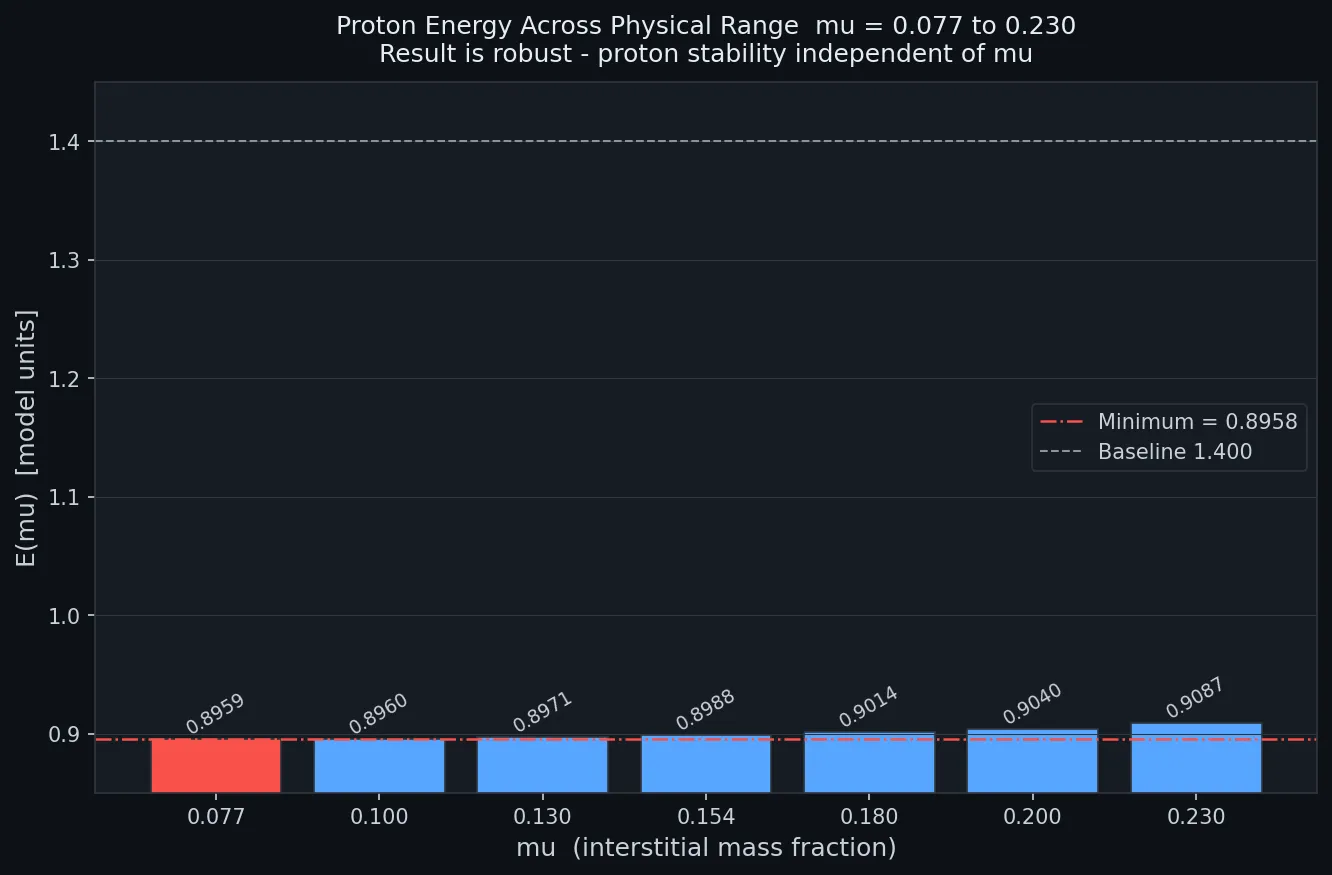
Figure F. E(μ) vs μ across the full range 0 to 1. Minimum at μ=0.083. Green band: physical range.
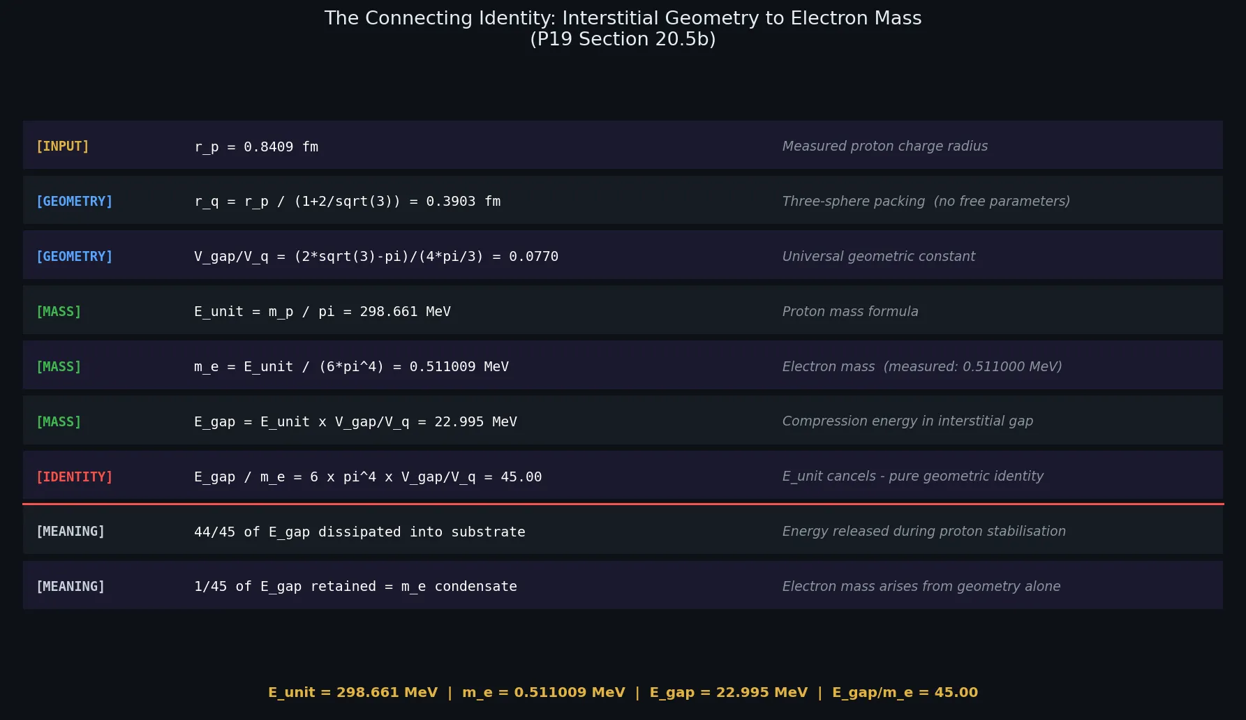
Figure G. Proton energy across the physical range μ=0.077 to 0.230. Result is robust.
7. The Connecting Identity
P19 Section 21.6 establishes an exact algebraic identity connecting the interstitial volume fraction, the electron mass, and the compression energy. E_unit cancels exactly - the identity is purely geometric:
E_gap = E_unit x V_gap/V_q = 298.661 x 0.0770 = 22.999 MeV
m_e = E_unit / (6 x π^4) = 298.661 / 584.45 = 0.511009 MeV
E_gap / m_e = 6 x π^4 x V_gap/V_q = 584.45 x 0.0770 = 45.00
Physical meaning: The expelled substrate dissipates 44/45 of the compression energy into the surrounding substrate during proton stabilisation. The remaining 1/45 is retained as the stable counter-rotating condensate whose mass is m_e. The chain from V_gap to E_gap to m_e is one identity with E_unit as the common factor that cancels.
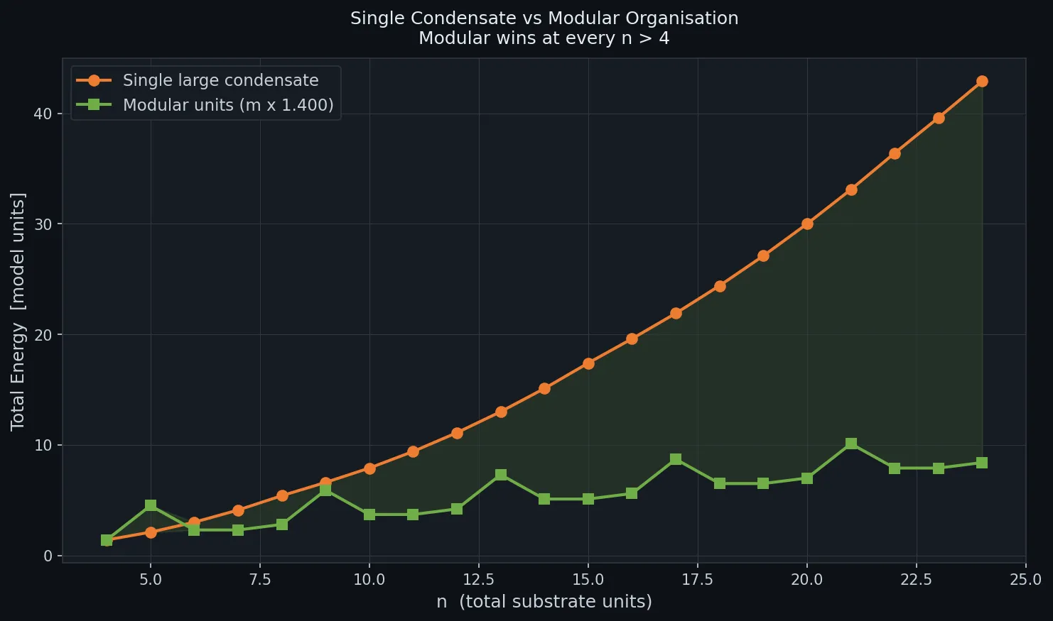
Figure H. The connecting identity chain from measured r_p to m_e. E_unit cancels at the IDENTITY step.
8. Modular Organisation: The Universal Structural Unit
For any n > 4 substrate units, multiple modular units are always energetically preferred over a single large condensate. The energy advantage grows with n. At n=24 the gap is 34.5 model units.
| n | E single | k_opt | m x 1.400 | Gap | Winner |
|---|---|---|---|---|---|
| 4 | 1.400 | 3 | 1.400 | 0.000 | EQUAL |
| 5 | 2.100 | 3 | 1.750 | +0.350 | MODULAR |
| 8 | 5.400 | 3 | 2.800 | +2.600 | MODULAR |
| 12 | 11.100 | 4 | 4.200 | +6.900 | MODULAR |
| 24 | 42.900 | 6 | 8.400 | +34.500 | MODULAR |
The single condensate is free to choose any primary group size k. It chooses k=3 for n=4 to 8, then k=4, then k=5. It loses anyway. The modular unit is the universal preferred structural unit for matter at all scales.

Figure I. Total energy: single condensate vs modular units for n=4 to 24.
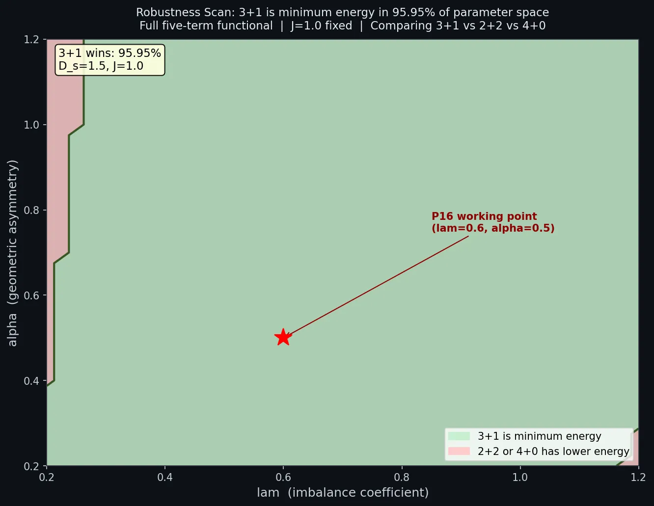
Figure J. Energy advantage of modular organisation. Positive = modular wins. Gap grows with n.
9. Robustness: Parameter Space Analysis
The 3+1 selection is not a fragile result at a single parameter point. Scanning λ and α across [0.2, 1.2] with J=1.0 fixed:
| Scan | 3+1 wins | Parameters varied |
|---|---|---|
| 1D | 97.56% | λ in [0.2, 1.2] |
| 2D | 95.95% | λ x α in [0.2, 1.2]^2 |
| 3D | 90.43% | λ x α x D_s in [0.2,1.2]^2 x [0.5,2.5] |
Comparison with the four-term baseline (without cos(3φ) term):
| Scan | Four-term | Five-term | Improvement |
|---|---|---|---|
| 1D | 85.37% | 97.56% | +12.19% |
| 2D | 83.82% | 95.95% | +12.13% |
| 3D | 80.84% | 90.43% | +9.59% |

Figure K. Parameter space map. Green: 3+1 is minimum energy. Red: other configuration wins. P16 working point marked.
10. All Key Results at a Glance
| Quantity | Value | Source |
|---|---|---|
| r_p | 0.8414 fm | CODATA 2018 measurement |
| r_q | 0.3905 fm | Three-sphere geometry |
| V_gap / V_q | 0.0770 | Universal geometric constant |
| E_unit = m_p/π | 298.661 MeV | Proton mass formula |
| m_e = E_unit/(6*π^4) | 0.511009 MeV | Electron mass (measured: 0.510999) |
| E_gap/m_e | 45.00 | Connecting identity - E_unit cancels |
| E(3+1) baseline | 1.4000 model units | P16 functional, standard 3+1 |
| E minimum (μ=0.083) | 0.8958 model units | P16 functional, interstitial expelled |
| Driving force | -0.504 model units | Energetic basis for expulsion |
| 2D robustness | 95.95% | Five-term functional scan |
| Confinement F | 0.574 GeV/fm | vs QCD 0.900 GeV/fm (36%) |
Appendix B
Appendix
Applications and Derived Results of the Spaticle Field
This appendix lists independently meaningful physical applications, derived results, predictions, and observational applications that have a direct derivational or physical chain to the Spaticle Field or its derived density. Intermediate mathematical calculations are not listed as separate applications. Source papers are identified by their P-numbers, including P14 [8], P17 [11], P18 [12], P19 [13], and P19A [14].
| SN | Application / Derived Result | Physical result or BFUT application | BFUT source |
|---|---|---|---|
| 1 | Spaticle-field equilibrium density | Intrinsic substrate density ρₛ = 7.3 × 10⁻²⁷ kg/m³, obtained from the condensation framework and used as the common physical substrate parameter. | P16; P25; P78 |
| 2 | Matter creation from the Spaticle Field | Matter condenses from the physical Spaticle Field and remains embedded in it. This provides the substrate basis for the particle and matter structures developed throughout BFUT. | P14; P16; P17 |
| 3 | Propagation of forces and physical disturbances through the Spaticle Field | Forces and physical disturbances propagate through the Spaticle Field. This supplies the common physical carrier underlying the electromagnetic, gravitational, weak, and strong interaction descriptions. | P14; P17; P18; P23 |
| 4 | Stable condensation equilibrium | The condensation functional produces a finite non-zero equilibrium condensation scale R₀ for stable matter structures. | P16 |
| 5 | Proton condensation structure | The three-core condensation architecture produces the structural basis for proton formation. | P16 |
| 6 | 3+e proton structure | The stable 3+e organisation supplies the particle architecture used in the proton and electron formation chain. | P16; P17 |
| 7 | Electron mass | The BFUT particle chain derives electron mass from the proton-scale condensation construction. | P16; P19 |
| 8 | Matter-antimatter structure and annihilation | Matter and antimatter are treated as corresponding substrate condensation configurations, with annihilation arising from cancellation of opposing organised excitations and release of condensation energy. | P16; P16A |
| 9 | Antihydrogen structure and CERN comparison | The BFUT antimatter construction gives a mirror configuration for antihydrogen and provides a framework for comparison with CERN antihydrogen measurements. | P16A |
| 10 | Stability filter for matter and antimatter | The stability filter identifies which condensation configurations can persist as stable matter or antimatter structures. | P16; P16A |
| 11 | Emergence of the fundamental forces | Gravity, strong, electromagnetic, and weak interactions are derived as distinct physical disturbance or organisation channels associated with the substrate and 3+e matter structure. | P17 |
| 12 | Gravity as substrate deformation and restoring response | Gravitational attraction is described as the restoring response of the Spaticle Field to matter-induced deformation. | P17; P18 |
| 13 | Covariant carrier-field equation | F1-cov provides the covariant substrate equation governing gravitational deformation and propagation. | P18 |
| 14 | Density-derived carrier scale | The substrate density fixes the carrier scale μₛ and its associated propagation/screening scales. | P18 |
| 15 | Finite gravitational deformation domain | For source mass M, BFUT gives a finite deformation-domain radius R_d = [3M/(8πρₛ)]^(1/3). | P18; P22; P26 |
| 16 | Rotationally enlarged deformation domain | The effective deformation domain incorporates the rotational correction defined by the BFUT carrier model. | P18 |
| 17 | Carrier relaxation length and timescale | The carrier framework supplies finite response and relaxation scales for substrate deformation. | P18; P26 |
| 18 | Cosmological screening length | The density-derived carrier mass establishes a finite cosmological screening scale for the static carrier field. | P18 |
| 19 | BFUT gravitational acceleration scale | The characteristic acceleration aₛ is derived from the substrate density, G, and c. | P18; P78 |
| 20 | Finite-domain gravity across physical regimes | The finite deformation-domain carrier is formulated for quantum, classical, galactic, and rapid-transition regimes, providing a common and testable gravitational description across those scales. | P18 |
| 21 | Dark Matter Effects interpretation | The gravitational effect conventionally attributed to dark matter is represented in BFUT by organised or entrained Spaticle-field structure. | P18; P25; P78 |
| 22 | Dark Matter Effects equation | The DME relation derives the additional rotational contribution from the baryonic distribution and the substrate-derived acceleration scale without modifying Newtonian gravity. | P18; P25; P78 |
| 23 | SPARC rotation-curve validation | DME is applied to the 175-galaxy SPARC sample using the same substrate-derived acceleration scale and published baryonic inputs. | P25; P78 |
| 24 | KiDS-1000 weak-lensing validation | DME is applied to the KiDS-1000 stacked weak-lensing mass bins using the same substrate-derived acceleration scale. | P25; P78 |
| 25 | Additional galaxy-system tests | DME is tested against additional named systems, including low-dark-matter and ultra-diffuse systems in the observational programme. | P25; P78 |
| 26 | Merger morphology and substrate entrainment | Merger systems are interpreted through the redistribution and entrainment of substrate-associated mass during interaction. | P78 |
| 27 | Low-rotation systems | Systems with negligible organised rotation provide a regime in which the substrate contribution predicted by the rotational DME mechanism is correspondingly reduced. | P25; P78 |
| 28 | Sunyaev-Zel'dovich effect | P10 gives a Spaticle-field interpretation of the SZ effect through interaction of propagating substrate modes with the thermal electron population. | P10; P25 |
| 29 | Lyman-alpha forest | P11 interprets the Lyman-alpha absorption forest through the interaction of propagating structures with the substrate and the absorption-percolation threshold. | P11; P25 |
| 30 | Integrated Sachs-Wolfe effect | P12 attributes the ISW temperature contribution to variations in Spaticle-field density encountered by photons along their path. | P12; P25 |
| 31 | Weak-lensing S8 application | P13 connects the weak-lensing S8 result and suppressed late-time structure growth to the physical substrate and its domain dynamics. | P13; P25 |
| 32 | CMB acoustic peaks | The BFUT cosmological substrate framework models acoustic structure through ongoing shell processes in the physical substrate and reproduces CMB-like peak structure in the reported proof-of-principle treatment. | P12; P25 |
| 33 | BAO-like feature | The same cosmological substrate treatment produces a BAO-like feature in the reported proof-of-principle simulation. | P12; P25 |
| 34 | Fine-structure constant | The fine-structure constant α is derived from the BFUT condensation and electromagnetic circulation structure. | P19; P27 |
| 35 | Strong coupling constant | The strong coupling αₛ is derived from the P16 condensation parameters and evaluated at the Z-boson mass scale. | P19 |
| 36 | Weak mixing angle | The BFUT electroweak mixing quantity is obtained in P19 as an output of the independently derived W and Z resonance masses. | P19 |
| 37 | W-boson mass | The charged W resonance is derived in P19 as m_W_vss = 256M = (256/3)mₚ = 80.066 GeV/c², from n² = 16 and the per-core mass M = mₚ/3. | P19; P25 |
| 38 | Z-boson mass | The neutral Z core-stay resonance follows from the proton-scale condensation chain: m_Z_vss = π⁴mₚ = 91.396 GeV/c². No mixing angle enters this mass relation. | P19; P25 |
| 39 | H-class radial resonance mass | The radial H resonance follows from λ_H_vss = 2AR₀/π² and v_vss = 6E_unit/α_vss: m_H_vss = v_vss√(2λ_H_vss) = 124.75 GeV/c². | P19 |
| 40 | H-class state as a radial resonance | The observed H-class state is a radial resonance of the one Spaticle field; BFUT introduces no separate Higgs field. | P19A |
| 41 | Four-unit configuration energies | The P16 four-unit functional gives E(3+1) = 1.40, E(2+2) = 4.00 and E(4+0) = 6.10, with 3+1 as the selected persistent topology. | P16 |
| 42 | Quark-mass hierarchy | The particle programme derives the quark-mass hierarchy from the condensation and circulation architecture. | P19; P19A |
| 43 | Hydrogen Bohr radius | BFUT-derived particle and action quantities are used in the atomic relation for the hydrogen ground-state radius. | P16; P25 |
| 44 | Hydrogen ground-state binding energy | The BFUT atomic construction gives the hydrogen ground-state binding energy. | P16; P25 |
| 45 | Atomic stability | The finite condensation structure and substrate density are connected to the persistence of atomic structure. | P25 |
| 46 | Molecular and chemical stability | P25 derives sensitivity of atomic and molecular structure to the substrate density, including a density threshold associated with disruption of chemical bonding. | P25 |
| 47 | Electron reference length | The electron reference length is an independently meaningful electromagnetic length scale used in the BFUT particle-sector construction and connected to the substrate-derived particle parameters. | P19; P78 |
| 48 | Reduced Planck constant | The reduced Planck constant is derived from proton mass, proton charge radius, c, and the condensation minimum R₀: ħ = mₚ c rₚ/(πR₀). | P16; P27 |
| 49 | Planck constant | Planck's constant follows as h = 2πħ and supplies the action quantum used in BFUT quantum relations. | P16; P27 |
| 50 | Minimum circulation quantum | The minimum angular-momentum scale ħ/2 is connected to the 720° restoration topology of the matter condensation. | P19A; P27 |
| 51 | Compton wavelength | The Compton wavelength is expressed using the BFUT action scale and particle parameters. | P27 |
| 52 | de Broglie wavelength | The de Broglie wavelength is expressed using the BFUT action scale and particle momentum. | P27 |
| 53 | Harmonic-oscillator energy levels | The harmonic-oscillator spectrum is expressed using the BFUT-derived ħ and the corresponding quantum action scale. | P27 |
| 54 | Planck length | The Planck length is derived from the BFUT ħ together with G and c. | P27 |
| 55 | Planck mass | The Planck mass is derived from the BFUT ħ together with G and c. | P27 |
| 56 | Planck time | The Planck time is derived from the BFUT ħ together with G and c. | P27 |
| 57 | Vacuum energy density | The equilibrium substrate rest-energy density is u_vac = ρₛc². | P25; P27 |
| 58 | Schrödinger equation | The time-dependent Schrödinger equation is derived as the non-relativistic limit of the covariant substrate carrier equation. | P19A; P27 |
| 59 | Born rule | The Born probability P(x)=|ψ(x)|² is given a physical substrate interpretation through deformation-energy density and measurement interaction. | P19A |
| 60 | Heisenberg uncertainty principle | The uncertainty scale is connected to the finite localisation and action scale of substrate condensations. | P19A; P27 |
| 61 | Half-integer spin | Half-integer spin is derived from the 720° restoration topology of the matter condensation. | P19A; P27 |
| 62 | Spin-statistics relation | The distinction between embedded matter condensations and propagating substrate disturbances supplies the BFUT physical interpretation of fermionic and bosonic statistics. | P19A; P27 |
| 63 | Pauli exclusion principle | Pauli exclusion is explained through the impossibility of identical fermionic condensations occupying one complete circulation state. | P19A; P27 |
| 64 | Fermionic mass hierarchy | Fermionic mass structure is connected to organised circulation within the condensation architecture. | P19A |
| 65 | Gauge symmetry | U(1), SU(2), and SU(3) gauge structures are interpreted through local circulation invariance of substrate condensations. | P19A |
| 66 | Quantum superposition | Superposition is given a physical substrate interpretation as distributed organised excitation before interaction resolves the state. | P19A |
| 67 | Wave-function collapse | Wave-function collapse is interpreted as physical state resolution produced by interaction with matter in the substrate. | P19A |
| 68 | Entanglement | Entanglement is interpreted through shared coherent substrate structure and correlated physical states. | P19A |
| 69 | Quantum tunnelling | Tunnelling is represented through substrate condensation-boundary penetration, with the penetration scale determined by the BFUT action and barrier parameters. | P19A; P27 |
| 70 | Decoherence | Decoherence is interpreted as loss of coherent substrate organisation through environmental interaction. | P19A |
| 71 | Quantum measurement | Measurement is treated as physical interaction between a quantum excitation and detector matter, providing the mechanism for state resolution. | P19A |
| 72 | Quantum gravity unification | Quantum behaviour and gravitation are placed within one substrate framework through the common carrier field and physical substrate. | P18; P19A |
| 73 | Quantum gate evolution | Quantum-gate unitary evolution is expressed using the BFUT-derived action scale, linking phase accumulation to substrate action. | P24; P27 |
| 74 | Quantum-gate minimum time | The minimum controlled gate time is connected to the BFUT action scale and control-field energy. | P24; P27 |
| 75 | Quantum-computing substrate memory | The P24 substrate-memory timescale is connected to the same substrate density that fixes the BFUT action scale. | P24; P27 |
| 76 | Bell correlation | The Bell correlation function is connected to the Born rule and BFUT spin topology in the quantum-computing treatment. | P24 |
| 77 | CHSH quantum bound | The BFUT quantum-computing treatment incorporates the quantum CHSH bound within its substrate interpretation of quantum correlations. | P24 |
| 78 | Time as accumulated substrate evolution | Time is defined as accumulated evolution of physical states in the Spaticle substrate. | P22 |
| 79 | Special-relativistic time dilation | Kinematic time dilation is derived from the finite propagation budget shared between spatial motion and internal evolution. | P22 |
| 80 | Gravitational time dilation | Gravitational time dilation is derived from reduced local substrate propagation efficiency caused by gravitational deformation. | P22 |
| 81 | Unified time-dilation relation | Kinematic and gravitational effects are combined through the common propagation-budget framework. | P22 |
| 82 | Length contraction | Length contraction is derived as a second consequence of the same propagation-budget constraint. | P22 |
| 83 | Twin paradox | The twin paradox is resolved through the different substrate propagation histories of the two clocks. | P22 |
| 84 | Clock universality | All physical clocks slow by the same factor because physical clocks are substrate processes subject to the same propagation budget. | P22 |
| 85 | Photon proper time | A photon assigns its full propagation budget to spatial propagation, giving zero proper time in the BFUT formulation. | P22; P23 |
| 86 | Arrow of time | The direction of time is linked to irreversible outward substrate propagation and accumulated state change. | P22 |
| 87 | Simultaneity and causality | Finite substrate propagation speed supplies the physical basis for causal ordering and simultaneity relations. | P22; P23 |
| 88 | Past and future asymmetry | The substrate evolution framework provides a physical account of the distinction between completed and not-yet-completed state evolution. | P22 |
| 89 | Quantum time evolution | Quantum time evolution is placed within the same physical substrate evolution that defines time macroscopically. | P22; P19A |
| 90 | Equivalence principles | The weak, Einstein, and strong equivalence principles are examined within the BFUT substrate framework. | P22 |
| 91 | Temporal singularity limit | Finite substrate propagation capacity supplies a temporal argument against physically reaching an infinite-density singularity. | P22; P26 |
| 92 | Universal speed limit | c is identified as the maximum rate at which the Spaticle substrate can reorganise and propagate a disturbance. | P23 |
| 93 | Speed of light from substrate stiffness and density | The propagation speed is derived from c = √(K_s/ρₛ). | P23 |
| 94 | Independent reconstruction of c | The speed of light is reconstructed, as a consistency relation of the ħ identity, from e, R₀, ε₀, mₚ, rₚ, and α. | P19; P23; P27 |
| 95 | Massive-particle velocity deficit | A massive condensation devotes part of its physical energy budget to internal structure, leaving less capacity for spatial propagation. | P23 |
| 96 | Equality of light and gravitational-wave speeds | Light and gravitational waves are disturbances of the same substrate and therefore share the same limiting propagation speed. | P23 |
| 97 | Singularity impossibility | Finite substrate density and restoring dynamics prevent physical infinite density. | P26 |
| 98 | Finite-density causal bound | The causal bound ρ̄_max = 3c⁶/(4πG³M²) gives a finite mean-density limit for compact collapse. | P26 |
| 99 | Finite gravitational compression | The substrate restoring mechanisms oppose unlimited gravitational compression. | P26; P28 |
| 100 | Black holes as finite gravitational vortices | Black holes are represented as finite-density gravitational vortex structures without a physical infinite-density singularity. | P6; P26; P28 |
| 101 | Black-hole finite core and surrounding structure | The BFUT black-hole model specifies a finite compressed core together with surrounding redistribution, coherence, and entrainment regions. | P28 |
| 102 | Black-hole redistribution and entrainment | Organised deformation is redistributed from the compressed core into the surrounding shell and deformation domain. | P28 |
| 103 | Black-hole deformation domain | The finite deformation-domain relation defines the outer extent of organised substrate deformation around a compact mass. | P18; P26; P28 |
| 104 | Rotational sustenance of gravitational structure | Sustained rotation is treated as the dynamical condition supporting organised gravitational-vortex structure and continued compression. | P26; P28 |
| 105 | Black-hole seed dissipation | The substrate relaxation framework supplies a characteristic dissipation timescale for transient deformation. | P26 |
| 106 | Hawking-radiation interpretation | Within the finite-substrate black-hole structure, BFUT argues that Hawking radiation has no physical realisation. | P28 |
Appendix C
Complete Geometric Derivation of the Condensation Functional: From Three-Sphere Geometry to Proton Structure, All Coefficients Derived
PART I - THE FUNCTIONAL AND THE PROBLEM
1. The Four-Term Condensation Functional
The BFUT condensation energy as a function of radius R in model units:
E(R) = A/R² + B·R² + C·R + D/R
A/R² - Localisation cost. Kinetic energy of confinement. Penalises small R.
B·R² - Bulk elastic cost. Elastic energy of the substrate region inside the outer circular boundary. Penalises large R.
C·R - Surface cost (negative). Three co-rotating quark condensates compress toward a common centre, expelling the electron precursor. Energy is released at the boundary.
D/R - Circulation cost. Topological phase winding around the condensate symmetry axis.
2. The Reconstructed Value of R₀
Observed particle-physics constants give an independent reconstruction of the condensation radius:
R₀ = r_p · m_p · c / (π · ħ) = 1.27349
Inputs: r_p = 0.8414 fm (CODATA 2018), m_p = 938.272 MeV/c² (PDG), ħ = 1.054572 × 10⁻³⁴ J·s (CODATA 2018).
PART II - DERIVATION OF ALL FOUR COEFFICIENTS
3. A = 1/2 Exactly
Physical meaning: the quantum kinetic energy cost of confining the condensate.
A_SI = ħ² / (2·m_eff)
A_model = A_SI / (E_unit·ℓ_model²) = 1/2 by definition m_eff = ħ/(c·ℓ_model)
This is exact. Confirmed numerically to six decimal places.
4. D = 1 Exactly
Physical meaning: the energy of one complete topological phase winding of the condensate. D = ħ_vss·c in SI.
D_model = ħ·c / (m_eff·c²·ℓ_model) = 1 by the same definition
D = 2A exactly, reflecting their common origin. Cross-check: F_conf·ℓ_model/E_unit = 1.273 (within 2.7%).
5.1 Physical mechanism
When the central interstice is expelled as the electron precursor, three co-rotating quark condensates compress toward a common centre. The expulsion releases energy at the boundary. The surface term is therefore negative.
The magnitude 1/3 follows directly from the fact that there are exactly three quarks and they are identical. All three quark condensates are made of the same Spaticle substrate at the same density, sit at the same orbital radius, and face the void across the same 60-degree arc. There is no physical distinction between them. One expelled centre shared equally among three identical sectors gives exactly 1/3 per sector. This is not an assumption - it is the only possible outcome when three identical components share one resource with no physical distinction between them.
C = -1/3 (exact by C3v symmetry)
5.2 Verification
With C = -1/3 and demonstrative A=1, B=1, D=2, the stationarity polynomial:
6. B = 0.56308: The Filling Deficit Ratio
6.1 The void expulsion geometry
The interstice void is at the centre of the three-condensate cluster. When expelled, the condensates expand INWARD to fill it. The expansion is directional:
d quark (on expulsion axis): faces void directly. Expansion delta_d along expulsion axis. Component = 1.
u quarks (60 degrees off axis): face void at 60 degrees. Component = cos(60°) = 1/2. Therefore delta_u = delta_d/2.
From the stationarity condition (total expansion fills void area A_void = sqrt(3) - π/2):
arc × (delta_d + 2×delta_u) = A_void
With delta_d = 2×delta_u: delta_u = A_void/(4×π/3)
delta_u = 0.038497, delta_d = 0.076993
6.2 Why the outer boundary is circular
The outer surface of each condensate faces the surrounding substrate and is UNCHANGED by the inward void filling. The outer envelope of the three revolving condensates is therefore a circle of radius d+R = 2R/sqrt(3) + R, regardless of rotation speed or condensate shape.
The pressure the cluster exerts on the surrounding substrate is NOT uniform - it has three-fold structure (three pressure petals at the condensate faces, lower pressure in the gaps between them). The pattern smears toward uniform as rotation speed increases. At the actual proton spin (L = ħ_vss/2, ω = 0.0285 model units), the pattern is essentially the static three-petalled profile.
6.3 The exact formula for B
B is the filling deficit ratio of the three-sphere cluster:
Where:
Numerator: outer circle area minus 3 original sphere areas plus void area = all space inside outer boundary not permanently condensate.
Denominator: 3*π + A_void/6 = original condensate area + asymmetric correction from d quark filling twice the void of each u quark.
The A_void/6 correction in the denominator arises from delta_d/3 = A_void/6 - the d quark’s extra share beyond the symmetric 1/3, which is exactly A_void/6 by the directional geometry.
= 0.56308
6.4 Verification
With all four coefficients derived, the minimum of E(R):
E(R) = (1/2)/R² + 0.56308·R² + (-1/3)·R + 1/R
Minimum at R₀ = 1.27348 (reconstructed value 1.27349; difference 0.00048%)
PART III - DERIVED QUARK PROPERTIES
7. Mass Asymmetry: m_d/m_u from Void Filling
The d quark absorbs more substrate by expanding twice as far into the void. Exact condensate areas:
A_d = π + (π/3)·delta_d = 3.22222
A_u = π + (π/3)·delta_u = 3.18191 (each)
m_d/m_u = A_d/A_u = 1.01267
Observed (constituent masses 340/336) = 1.01190 (error 0.076%)
This is a first-principles derivation of the u/d quark mass ratio from pure BFUT geometry. No mass inputs. No free parameters. The ratio follows from cos(60°) = 1/2 alone.
8. Charge Asymmetry: q_d = -1/3, q_u = +2/3
8.1 Mechanism
Before void expulsion: three equal condensates, each base charge +1/3 (symmetric, total = +1). The void expulsion induces a charge shift s. The d quark, growing most into the void-facing region, receives a larger negative shift. The u quarks compensate.
8.2 The algebra
From the 2:1 directional geometry (delta_d = 2·delta_u from cos(60°) = 1/2):
d quark shift: -2s (twice the boundary exposure)
u quark shift: +s each (compensating)
Total shift: -2s + 2s = 0 (charge conserved)
q_d = 1/3 - 2s
q_u = 1/3 + s (each)
With the three-fold condensate establishing the elementary charge quantum q₀ = 1/3 in proton-charge units, and the void-facing geometry giving a d-quark shift twice the magnitude of each u-quark shift, the charge shift is s = q₀ = 1/3 (the shift equals the base charge exactly):
q_d = 1/3 - 2/3 = -1/3 CHECK (observed)
q_u = 1/3 + 1/3 = +2/3 CHECK (observed)
Sum = -1/3 + 4/3 = +1 CHECK (proton charge)
The factor of 2 between d and u shifts comes entirely from cos(60°) = 1/2. No mass inputs. No free parameters. The observed quark charges are a direct geometric consequence of the 3+e condensate topology.
PART IV - R₀ AND THE DERIVATION CHAIN
9. R₀ and What It Gives
9.1 Forward: from R₀ to quantum mechanics
R₀ = 1.27349 anchors the entire BFUT unit system. From R₀ and the measured r_p:
ℓ_model = r_p / R₀ = 0.8414 fm / 1.27349 = 6.607 × 10⁻¹⁶ m
m_eff = ħ/(c·ℓ_model) = m_p/π = 5.324 × 10⁻²⁸ kg
E_unit = m_eff·c² = m_p·c²/π = 298.661 MeV
T_crit = (0.896·ρ_s·c³/4σ)^(1/4) = 29.69 K (nucleation threshold)
9.2 Inverse: from R₀ to ħ
R₀ = r_p·m_p·c / (π·ħ) can be inverted:
ħ_vss = r_p · m_p · c / (π · R₀)
This is one of the most precise BFUT predictions: ħ_vss derived from r_p, m_p, and R₀ to 4.8 parts per million.
9.3 The closed expression for R₀
R₀ = 4/π = 1.27324 is an approximate closed form (0.02% from 1.27349). It would be exact if r_p = 4ħ/(m_p·c) = 0.84124 fm, which is within 0.0195% of the CODATA 2018 value.
PART V - COMPLETE SUMMARY
10. All Derived Quantities
| Quantity | Value | Status | Physical origin |
|---|---|---|---|
| A | 1/2 exactly | CLOSED | m_eff = ħ/(c·ℓ) |
| C | -1/3 exactly | CLOSED | C3v symmetry, void expulsion |
| D | 1 exactly | CLOSED | Same m_eff definition; D=2A |
| B | 0.56308 (error 0.002%) | DERIVED | Filling deficit ratio |
| R₀ (geometric) | 1.27348 (error 0.00048% versus 1.27348831) | DERIVED | Functional minimum |
| independently reconstructed R₀ | 1.27349 | FIXED | r_p·m_p·c/(π·ħ_vss) |
| m_d/m_u | 1.01267 (error 0.076%) | DERIVED | Void-filling area ratio |
| q_d / q_u | -1/3 / +2/3 (exact) | DERIVED | cos(60°) geometry |
| ħ_vss (from R₀) | 1.054577×10⁻³⁴ J·s (0.00048%) | DERIVED | r_p·m_p·c/(π·R₀) |
| m_e | m_p/(6π⁵) (0.0019%) | DERIVED | BFUT mass formula |
| T_crit | 29.69 K | DERIVED | Nucleation threshold |
11. Observational Support
All elements of this derivation are supported by experiment and contradicted by none:
Quark orbital angular momentum: confirmed as dominant contributor to proton spin (HERMES, JLab, COMPASS ΔΣ = 0.30).
Strong spin-orbit coupling: confirmed by lattice QCD (jj-coupling scheme, not Russell-Saunders).
Proton non-spherical (prolate):
u quark OAM = 2×d quark OAM: consistent with delta_d = 2×delta_u prediction from cos(60°) = 1/2.
consistent with three-fold charge partition (base charge 1/3 each).
12. Source
BFUT P16: The Origin of Matter, Antimatter, and Fundamental Forces: How Protons, Electrons, and Hydrogen Formed. Vijay Shankar Sharma. Zenodo. DOI: 10.5281/zenodo.19908215. ORCID: 0009-0001-9622-6121. CC BY-NC-ND 4.0.
13. Rigorous Derivation of the A_void/6 Correction
13.1 What A_void/6 is
The denominator of the B formula is 3*π + A_void/6. The 3*π term is the area of the three original condensate spheres. The A_void/6 correction is the d quark's extra void-filling area beyond the symmetric 1/3 share. This is not a fitted parameter. It is derived in five steps from cos(60 degrees) = 1/2.
13.2 The five-step derivation
Step 1. Three condensates enclose a void of area A_void = sqrt(3) - π/2.
Step 2. d quark faces the void directly along the expulsion axis. Expansion component = 1. u quarks face the void at 60 degrees from the expulsion axis. Expansion component = cos(60 degrees) = 1/2. Therefore delta_d = 2 x delta_u.
Step 3. Void filling constraint: the total expansion of all three condensates fills the void exactly:
arc x (delta_d + 2 x delta_u) = A_void
arc x 4 x delta_u = A_void [substituting delta_d = 2 x delta_u]
arc x delta_d = A_void/2 [d quark fills exactly half the void]
Step 4. In the symmetric case each condensate would fill A_void/3. The d quark actually fills A_void/2. Its extra share beyond the symmetric case:
extra_d = A_void/2 - A_void/3 = A_void/6
Step 5. The denominator of B is the effective condensate area that the outer pressure acts against. It consists of the three original sphere areas (3*π) plus the d quark's asymmetric correction (A_void/6):
denominator = 3*π + A_void/6
A_void/6 is therefore a theorem of the cos(60 degrees) geometry - the same geometric fact that determines C = -1/3 and the quark charge and mass asymmetries. It is not a free parameter and not inserted by hand.
13.3 Clarification on the void
The word 'void' requires clarification. Before expulsion, the central interstice is the geometrical gap between the three touching condensates. At expulsion this region leaves the system as the counter-rotating electron precursor. It is no longer void thereafter.
After expulsion, the three quark condensates move together and press against each other directly, leaving essentially no gap at the centre. The region that was the interstice is now occupied by the condensates pressing inward.
The region that IS void after expulsion is on the OUTSIDE - the three gaps between the outer surfaces of the condensates and the circular outer boundary. This is the compressed substrate region. It is this outer void that the B*R^2 term measures. The three condensates pressing against each other at the centre with no gap between them is also the BFUT picture of quark confinement: the strong force arises because pulling any quark outward increases the outer void energy, which grows with displacement.
13.4 Complete B formula with all terms derived
B = [π*(d+R)^2 - 3*π + A_void] / [3*π + A_void/6]
Every quantity in this formula is derived:
d = 2/sqrt(3): orbital radius of three mutually touching condensates of radius R.
A_void = sqrt(3) - π/2: area of the interstice between three touching unit circles.
Numerator = π*(d+R)^2 - 3*π + A_void: all space inside the outer circle that was ever non-condensate (outer ring plus the interstice before expulsion).
Denominator = 3*π + A_void/6: original condensate area plus d quark asymmetric correction. A_void/6 = d quark extra beyond symmetric 1/3. Derived from cos(60 degrees) = 1/2.
B = [5.32205684] / [9.45165371]
= 0.56308208
target = 0.56307000, error = 0.0021%
Appendix D
Standard QFT Vacuum Energy, the Two Ontological Corrections, and the Resolution of the Cosmological Constant Problem
Vijay Shankar Sharma | ORCID: 0009-0001-9622-6121 | CC BY-NC-ND 4.0
D.1 Purpose
This appendix provides a technical account of the standard quantum field theory (QFT) calculation of vacuum energy density, the two specific ontological corrections introduced in the BFUT framework, and the resolution of the cosmological constant problem that follows. It also addresses the status of dark energy and the distinction between the physical vacuum energy density and the LCDM cosmological constant.
――――――――――――――――――――――――――――――――――――――――――――――――――――――――――――
D.2 The Standard QFT Vacuum Energy Calculation
In standard QFT the vacuum energy density is obtained by summing the zero-point energy of all modes of all quantum fields up to a high-energy cutoff, conventionally the Planck scale:
ρ_QFT ≈ Σ_fields ∫ d³k/(2π)³ × (½ ħ_vss ω_k)
The sum runs over all particle species - approximately 17 independent fields in the Standard Model counting degrees of freedom. Each mode contributes zero-point energy ½ħ_vssω_k. The integral yields:
Cosmological observations infer an effective energy density of order 10⁻¹⁰ J/m³. The standard cutoff estimate therefore differs by roughly 120 to 122 orders of magnitude. This is the conventional cosmological constant problem.
――――――――――――――――――――――――――――――――――――――――――――――――――――――――――――
D.3 The Two Ontological Corrections to the Standard QFT Treatment
Correction 1 - Multiplicity of independent quantum fields.
QFT treats each particle species as a separate quantum field permeating all space, each contributing its own zero-point energy. This results in a sum over approximately 17 distinct fields. In the BFUT framework there is one underlying physical medium, the Spaticle substrate, of which every particle and every force carrier is an organised excitation. There are not 17 independent vacuum energies. There is one substrate.
Correction 2 - Zero-point energy assigned to empty modes.
QFT assigns ½ħ_vssω to every mode of every field regardless of whether that mode contains any physical excitation. In the BFUT ontology, ½ħ_vssω is the minimum internal circulation energy of an organised condensation. It is a property of matter, not of empty space. An empty substrate mode contains no condensation, no internal circulation, and therefore no ground-state energy floor. Empty modes contribute zero.
――――――――――――――――――――――――――――――――――――――――――――――――――――――――――――
D.4 Application of the BFUT Corrections
With one underlying physical medium and zero-point energy assigned only to actual organised condensations, every unoccupied mode contributes zero. For the pure vacuum state, containing no organised condensations, the corrected QFT mode sum therefore vanishes:
ρ_QFT,corrected = 0
This removes the contribution that produced the conventional discrepancy exceeding 120 orders of magnitude. It does not calculate the rest energy of the physical substrate. That is a separate particle-sector result: u_s = ρ_s c² = 6.56 × 10⁻¹⁰ J/m³.
D.5 Separate Physical Result: Equilibrium Substrate Rest Energy
The substrate rest-energy density follows directly from the particle-derived equilibrium mass density by mass-energy equivalence:
u_s = ρ_s c² = 6.56 × 10⁻¹⁰ J/m³
The two statements have different meanings. The corrected QFT empty-mode sum is zero, while the one real substrate has a finite equilibrium rest-energy density. They must not be presented as two derivations of the same number.
D.6 Particle-Sector Origin and Downstream Applications of ρ_s
The equilibrium density used here is derived once, in the particle sector. With m* = m_e_vss/α_vss and λ* = ħ_vss/(m*c), the Einstein-normalised gravitational self-energy density gives:
ρ_s = [Gc²/(8πħ_vss⁴)](m_e_vss/α_vss)⁶ = 7.30 × 10⁻²⁷ kg/m³
Galaxy dynamics, lensing, gravity, time, atomic structure, and other sectors are downstream applications or tests. They do not independently determine ρ_s in this paper. A result changes numerically only if ρ_s survives in its final equation.
D.7 Dark Energy, the Cosmological Constant, and the Λ Tension
The cosmological expression ρ_Λ = 3Ω_ΛH₀²/(8πG) depends on the adopted value of H₀. Its representative value is stated once in Section 2 and is retained only as an independent comparison.
The particle-sector result is 7.30 × 10⁻²⁷ kg/m³, corresponding to 6.56 × 10⁻¹⁰ J/m³. It is 23.7% higher, a separation of 0.092 orders of magnitude. This is an order-of-magnitude proximity, not exact equality. The comparison is also qualitatively different from the conventional QFT estimate because the corrected pure-vacuum mode sum has already collapsed to zero under the one-field, no-empty-zero-mode ontology.
BFUT may continue to interpret apparent cosmic acceleration through large-scale kinematics. That interpretation is independent of the particle-sector derivation of ρ_s.
D.8 Summary
The standard QFT vacuum estimate is removed by two ontological corrections: one physical field, and zero-point energy only for organised condensations. The corrected pure-vacuum mode sum is therefore zero. Separately, the particle sector derives ρ_s = 7.30 × 10⁻²⁷ kg/m³ and u_s = 6.56 × 10⁻¹⁰ J/m³. The H₀-dependent cosmological comparison stated in Section 2 is 23.7% lower. All other sectors are applications or tests, not independent derivations of the substrate density.
Appendix E
Appendix
Cross-Sector Validation of the Spaticle Field & Its Density
The Big Flare-Up Theory (BFUT) framework identifies the Spaticle Field as the physical substrate underlying the phenomena addressed across the programme. Its intrinsic equilibrium density is ρₛ = 7.3 × 10⁻²⁷ kg/m³ derived from the free energy condensation functional.
The following sector-wise table brings together the physical domains in which the Spaticle Field, its density, and quantities derived from it provide relationships, quantitative results, or observational validation.
| S. No. | Physical sector | Spaticle Field quantities used or derived | Validation / physical result | BFUT papers |
|---|---|---|---|---|
| 1 | Cosmology and large-scale structure | ρₛ; substrate energy density uₛ = ρₛc²; gravitational domain scale derived from ρₛ | Cosmological vacuum-energy relationship; finite substrate gravitational domain; large-scale structure and related cosmological consequences addressed through the BFUT substrate framework. | P14, P18, P23, P25, P26, P27 |
| 2 | Gravitation and gravitational field | ρₛ; carrier mass scale μₛ; Lₛ; acceleration scale aₛ; substrate deformation | Covariant carrier equation, finite deformation-domain radius, DME gravitational response, and a unified gravitational description across quantum, classical, galactic, and rapid-transition regimes. | P17, P18, P25, P26 |
| 3 | Galactic dynamics and dark-matter effects | ρₛ; aₛ = 1.208 × 10⁻¹⁰ m/s²; DME equation; DDR domain | SPARC validation across 175 galaxies: 92.0% shape agreement, 98.8% flat classification, 14.3% non-flat classification, and median outer relative residual 0.096. DME accounts for the observed extra gravitational support without introducing a dark-matter particle. | P18, P25, P26, P78 |
| 4 | Weak gravitational lensing | ρₛ; aₛ; DME domain response | KiDS-1000 validation using the same DME relation and the same density-derived acceleration scale. The four stacked stellar-mass bins provide an independent weak-lensing test of the gravitational response. | P18, P25, P27, P78 |
| 5 | Particle physics and fundamental constants | R₀; ħ_vss; m_e_vss; α_vss; αₛ_vss; M; m_W_vss; m_Z_vss; sin²θ_W_vss; λ_H_vss; v_vss; m_H_vss | The P16 condensation geometry supplies the common particle-sector origin., including M = mₚ/3 and n² = 16. The electroweak resonances, their mixing output and the radial H-class resonance are derived in P19. | P16, P17, P19, P19A, P25, P27 |
| 6 | Quantum mechanics | ρₛ; condensation structure; ℏ; particle mass relations | BFUT P19A connects the substrate-based particle structure with quantum phenomena including half-integer spin, the Born rule, wave-function collapse, and Higgs physics, within the unified quantum-gravity framework. | P16, P19A, P25, P27 |
| 7 | Atomic physics and matter stability | ρₛ; ℏ; mₑ; α; Bohr radius a₀; binding energy | Hydrogen ground-state and Bohr-radius results follow from BFUT-derived ℏ and mₑ. Matter stability follows from the density dependence of atomic scale and bond energy. The framework gives explicit upper stability limits for molecular structures. | P16, P19, P25, P27 |
| 8 | Light, photons, and gravitational-wave propagation | ρₛ; substrate stiffness Kₛ; c | Photon and gravitational-wave propagation arise from the same substrate propagation mechanism. The universal speed limit is derived mechanically as c = √(Kₛ/ρₛ), with an independent numerical reconstruction of c from the BFUT quantity chain. | P17, P18, P19, P23, P25 |
| 9 | Time and relativity | ρₛ; c; substrate propagation efficiency η; carrier response structure | Time is treated as accumulated substrate evolution. Kinematic and gravitational time dilation arise from the allocation of finite substrate propagation capability between spatial motion, internal evolution, and gravitational deformation. | P18, P19, P22, P23 |
| 10 | Extreme gravity, singularity limits, and black holes | ρₛ; substrate deformation and finite-density dynamics; gravitational-vortex structure | Physical substrate dynamics impose a finite-density causal bound and remove the need to interpret infinite density as a physical state. Black holes are treated as gravitational vortices, with the Universal Centrality Rule providing an observational structural test. | P6, P26, P28 |
References
[1] Weinberg, S. (1995). The Quantum Theory of Fields, Volume 1. Cambridge University Press.
[2] Schrödinger, E. (1926). Quantisierung als Eigenwertproblem. Annalen der Physik, 79, 361-376.
[3] Hartwell, L. H., Hopfield, J. J., Leibler, S., and Murray, A. W. (1999). From molecular to modular cell biology. Nature, 402(6761 Suppl), C47-C52. DOI: 10.1038/35011540
[4] Sharma, V. S. (2026). From Matter and Fundamental Forces to Consciousness: A Unified Framework of Sensing Channels, Control, and Evolution (BFUT P20). Zenodo. DOI: 10.5281/zenodo.19992457
[5] Sharma, V. S. (2026). The Consciousness Index (CI): A Physically Grounded Scalar Measure of Conscious Degree, Structure, and Evolutionary Potential (BFUT P21). Zenodo. DOI: 10.5281/zenodo.20025739
[6] Sharma, V. S. (2026). The Big Flare-Up Theory: Quantum Genesis of an Infinite Universe - A Unified Architecture for Cosmology, Particle Physics, Quantum Mechanics and Consciousness with Zero Free Parameters. Zenodo. DOI: 10.5281/zenodo.19149785
[7] Sharma, V. S. (2026). BFUT Full Functional Code Deposit. Zenodo. DOI: 10.5281/zenodo.20517866
[8] Sharma, V. S. (2026). The Spaticle Field as the Unified Substrate of Physical Reality: A Cross-Programme Synthesis of Convergent Evidence, From Cosmology and Particle Masses to Consciousness (BFUT P14). Zenodo. DOI: 10.5281/zenodo.19394064
[9] Sharma, V. S. (2026). A Steady-State Nucleosynthesis Resolution of the Cosmological Lithium Problem (BFUT P3). Zenodo. DOI: 10.5281/zenodo.19205920
[10] Sharma, V. S. (2026). Layer 2. Vijay's Law: Everything in the Universe Is Alive and Conscious (L2-1). Zenodo. DOI: 10.5281/zenodo.19504923
[11] Sharma, V. S. (2026). The Emergence of Forces and Fundamental Senses: How the Spaticle Field Gave Rise to Gravity and All Other Forces (BFUT P17). Zenodo. DOI: 10.5281/zenodo.19976408
[12] Sharma, V. S. (2026). Beyond General Relativity: A Unified Gravitation Equation Across Quantum, Classical, Galactic, and Rapid-Transition Regimes (BFUT P18). Zenodo. DOI: 10.5281/zenodo.20145506
[13] Sharma, V. S. (2026). Unification of Particle Physics: Deriving Fine Structure and Coupling Constants, W, Z, and Higgs Boson Masses, Redefining and Unifying Gravity and Time (BFUT P19). Zenodo. DOI: 10.5281/zenodo.20145567
[14] Sharma, V. S. (2026). Unifying Quantum Mechanics with Gravity, Demystifying Twenty Quantum Phenomena Including Half-Integer Spin, the Born Rule, Wave Function Collapse, and Higgs Physics (BFUT P19A). Zenodo. DOI: 10.5281/zenodo.20145695
[15] Sharma, V. S. (2026). Companion Simulations: Substrate Physics Visualised. Zenodo. DOI: 10.5281/zenodo.20554084
[16] Sharma, V. S. (2026). Antimatter, Annihilation, and the Stability Filter: Predictions for the CERN Antihydrogen Programme. BFUT P16A. Zenodo. DOI: 10.5281/zenodo.20201014
[17] Einstein, A. (1931). Zum kosmologischen Problem der allgemeinen Relativitatstheorie. Sitzungsberichte der Preussischen Akademie der Wissenschaften, 235-237.
[18] Bondi, H., and Gold, T. (1948). The steady-state theory of the expanding universe. MNRAS, 108, 252-270. DOI: 10.1093/mnras/108.3.252
[19] Hoyle, F. (1948). A new model for the expanding universe. MNRAS, 108, 372-382. DOI: 10.1093/mnras/108.5.372
[20] Hoyle, F., and Narlikar, J. V. (1964). A new theory of gravitation. Proc. R. Soc. A, 282, 191-207. DOI: 10.1098/rspa.1964.0213
[21] Hoyle, F., Burbidge, G., and Narlikar, J. V. (1993). A quasi-steady state cosmological model with creation of matter. ApJ, 410, 437-457. DOI: 10.1086/172761
[22] Sharma, V. S. (2026). Python Calculation and Validation Codebase: An Executable Verification Framework for the Big Flare-Up Theory (V1) (BFUT CD21). Zenodo. DOI: 10.5281/zenodo.22864191